ABSTRACT
Diamonds used in jewellery represent the quintessential fusion of aesthetic appeal and technical expertise. Not only does it require extreme skill to cut a diamond, analyzing and predicting a diamond’s Visual Performance™ is essentially a technical mathematical problem. In particular, diamonds and other faceted gems have the property that they fragment the visual field into a set of polygons called virtual facets, which represent equivalence classes of light paths according to their facet interactions with the gem polyhedron.
In this paper we explain how this mathematically elegant conception forms a framework from which to analyze a diamond’s appearance and beauty. We intend this framework to form the foundation for a fancy-shaped diamond cut grading system.
Although virtual facet patterning has been studied before, mostly in the context of round brilliant diamonds, a significant new feature of our approach is to take into account the effect varying visual depths of virtual facets has on visual perception. We also showcase some novel designs created by our team at GIA using a mathematical enumeration algorithm for symmetric diamond-like polyhedra.
KEYWORDS
Virtual Facet Pattern (VFP), diamond design, light performance, crushed ice, bow-tie effect, girdle reflection, scintillation, fire, fancy cut diamonds, diamond visualization, optical modeling, lighting environment, dark zoning, ASET analysis, computer simulation, diamond cut evaluation.
INTRODUCTION
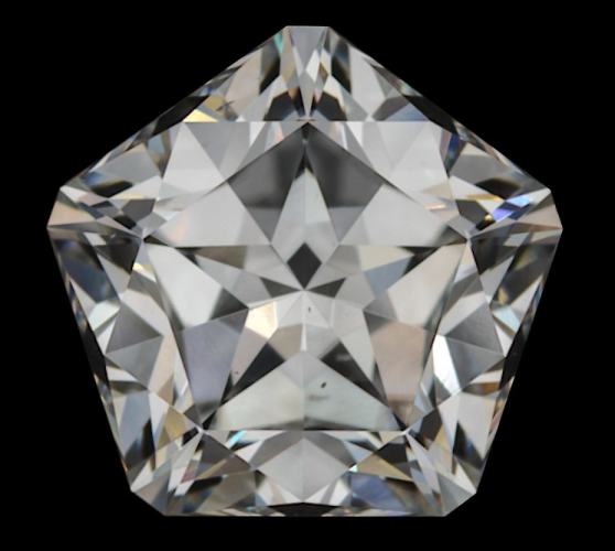
Consider the diamond images in Figure 1. The geometric patterns that we see are more complex than the simple surface faceting of the diamonds, representing nontrivial light paths through the gemstone. These patterns of virtual facets (VF), also called “mosaic patterns,” represent an essential visual and aesthetic quality of diamonds. The standard round brilliant diamond typically displays a pattern with moderate-to-small sized virtual facets. Among fancy shapes (any shape which is not a standard round brilliant), some cuts display large blocky virtual facets, while others show an even distribution of very fine virtual facets. Areas of very tiny virtual facets are often called “crushed ice,” named for the similarity to the sparkles of light one might see in actual crushed ice. Most fancy shaped diamonds produce patterns which have both regions of crushed ice and larger virtual facets.
Diamond designers are adept at creating virtual faceting patterns (VFP) in diamonds. One popular style of round brilliant shows a classic eight fold “arrow” pattern face-up, as seen in the leftmost diamond in Figure 1. Designers have also created stars (e.g. Figure 2), flower shapes, and more, with different diamond faceting arrangements.
VF patterns include a variety of features that designers aim to manipulate. The distribution of VF sizes is the most obvious. The dynamic play of crushed ice as the diamond moves and the juxtaposition of virtual facets at different optical depths are other factors for the designer to consider.
In other words, the task of the diamond designer is to get the virtual facet tessellation to produce a particular appearance, even if they don’t necessarily conceptualize it in those terms.
Creating a particular type of virtual facet pattern is not an easy task, because it is not obvious or intuitive how a particular faceting arrangement and proportion set will affect the face-up virtual facet view. Historically, particular cuts were arrived at through trial and error, while in the present day computer modeling is used.
In this paper, we discuss the basic mathematics and physics that explain how virtual facet patterns arise, including details of how we use computer modeling with forward and reverse ray and beam tracing. In particular we explain the creation of the polygonal tessellation by virtual facets and the calculation of where each virtual facet draws light from the environment. This can be accomplished via reverse ray or beam tracing using the so called primary ray approximation, which is sufficient for many modeling purposes. We explore the assumptions underlying this approximation: when they are reasonable, and when they need to be adjusted. In particular, we make the case that secondary rays play a fundamental role in many situations as well.
Diamond appearance has long been described in terms of brilliance (or brightness), referring to the visual impact of white light, fire, referring to observable colored light, and scintillation, referring both to sparkliness and how the VF pattern changes with motion. (Liddicoat, 1993) We present two model lighting environments useful for exploring various details of a diamond’s VFP that relate to these appearance qualities: models for diffuse lighting and spot lights.
Reverse ray tracing is sufficient for aspects explored in diffuse lighting, including windowing (an effect from ray paths straight through the diamond, also called leakage). Under spot lighting conditions, forward ray tracing is also useful, particularly for the analysis of fire (see Section 8).
We review and introduce several methods for coloring virtual facet patterns to give information about a diamond’s performance, and the use of these colorings for finding advantageous geometric
parameters for a given diamond cut. We also consider maps and analyses of all light directions surrounding a diamond (called the celestial sphere when set at infinite distance) in order to assess its visual qualities, especially with respect to scintillation. We finish by considering several examples of novel diamond cuts created using the enumeration algorithm developed in Conant (2024), interpreting their look and style through the lens of virtual facet analysis.
Cut analysis of diamonds through mathematical and computer modeling has a long history. We draw particular attention to Whitlock (1917), who did some of the first explicit ray tracing analysis without aid of a computer. In addition to the many papers cited in the body of this text, we also mention Tolkowsky (1919), Harding, Dodson (1979), Kato (1982), and Cowing (2009), though this list is by no means exhaustive. OctoNus has a webpage dedicated to diamond cut research as well. (Octonus Website, undated)
We note that the mathematical and computer modeling of diamond performance is a separate (though related) problem from that of photorealistic rendering of diamonds.
Remark 1. Our intention in this paper is twofold. The first is to give the interested technically-minded reader a sufficiently detailed account of the mathematics underlying the analysis of diamond cut for them to appreciate the beauty underlying this research area. The second is to establish technical details underlying a GIA (Gemological Institute of America) fancy cut grade system to be released in the near future. Thus our intended audience includes mathematicians and other non-diamond people who may find this subject, outside their normal purview, interesting, as well as diamond industry professionals who wish to understand more about how diamond optics work and how the GIA research group approaches the analysis. Bearing these two intended audiences in mind, we have tried to present the results with enough rigor to communicate the technical ideas effectively, while at the same time trying to keep the text readable to as wide an audience as possible.
Remark 2. The first few sections of this paper, outlining the basic mechanics of virtual facet patterns, are expository. The concept and mechanism of virtual facets was introduced in Sasian et al. (2007). However, the analytical frameworks, with the exception of the ASET and ALGW maps, are all new to this paper. Section 4 giving a rigorous mathematical definition of virtual facets, Section 5.1 on dual ASETs, Section 5.2 on virtual facet influence, Section 6 on focal distance and k-flector maps, Section 7.4 on girdle reflection, Section 8.1 on sparkle probability, Section 8.2 on sparkle spread, and Section 8.3 on fire, are all novel. Moreover the diamond cuts presented in Section 9 are all new GIA designs.
2. THE SOURCE OF VIRTUAL FACETS
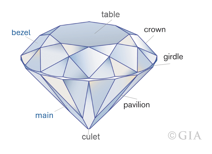
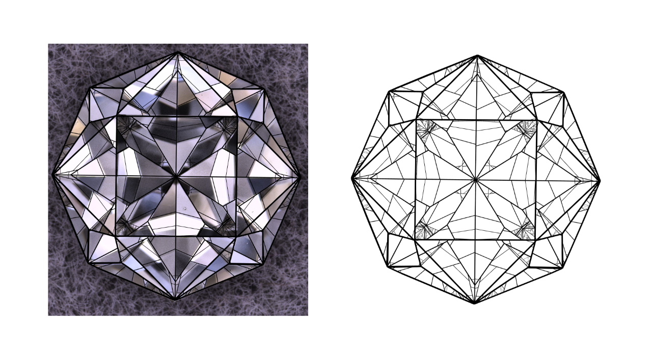
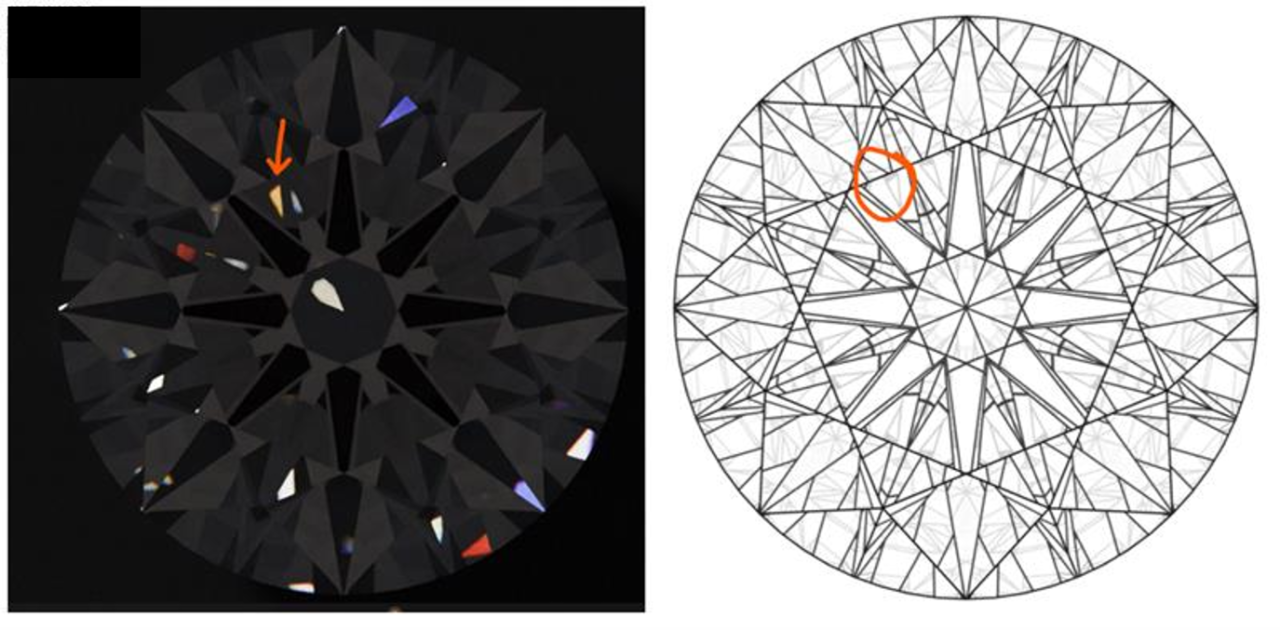
When one looks at a diamond, there is a lot more apparent structure than is accounted for by its faceting diagram. Figure 3 gives the gem-industry terminology for the parts of a polished diamond. A typical representation of this three dimensional geometry shows the crown and pavilion faceting projected into a horizontal plane. In Figure 4, we have a photo of a diamond and right next to it is a diagram of its crown faceting pattern. One can see that the actual visual pattern is more complicated than this diagram, subdividing each facet into smaller polygons. We call these virtual facets. Figure 5 shows a computer model of how these look, overlaid on the actual cut stone.
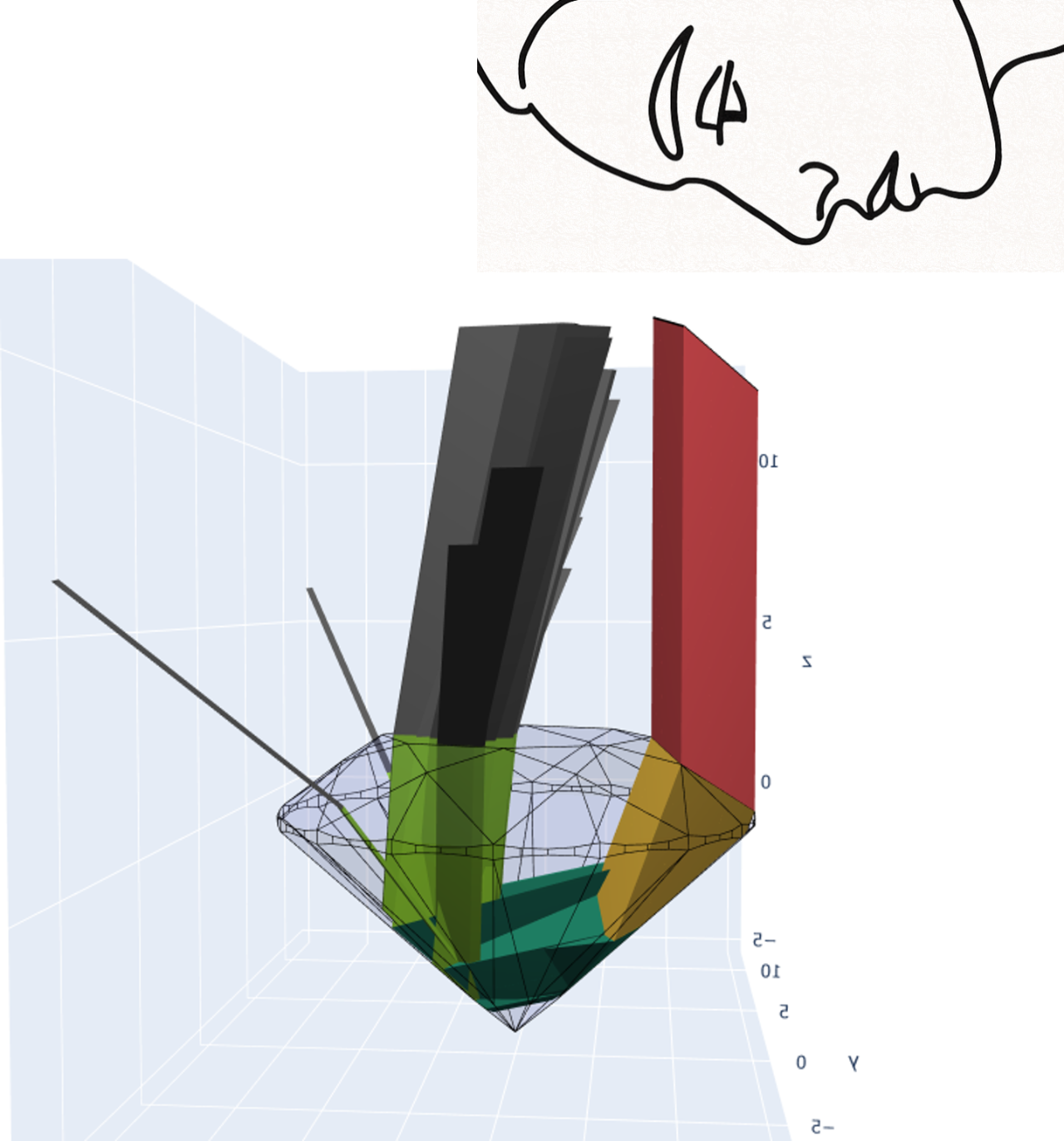
Consider a top-down view of a standard round brilliant diamond as in the left side of Figure 6. Let’s trace the portion of light coming from the shaded crown facet back through the diamond to see from where it originated in the environment. In the middle picture you see a side view of the beam, which fragments into many subbeams as it is traced backward, one per virtual facet. It reflects twice off the pavilion and then back out toward the table. Each time the beam hits the diamond’s surface, it fragments into smaller beams. Although messier to draw, one could visualize a single large beam reverse traced into the diamond crown, which then fragments into one subbeam per virtual facet.
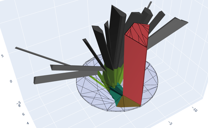
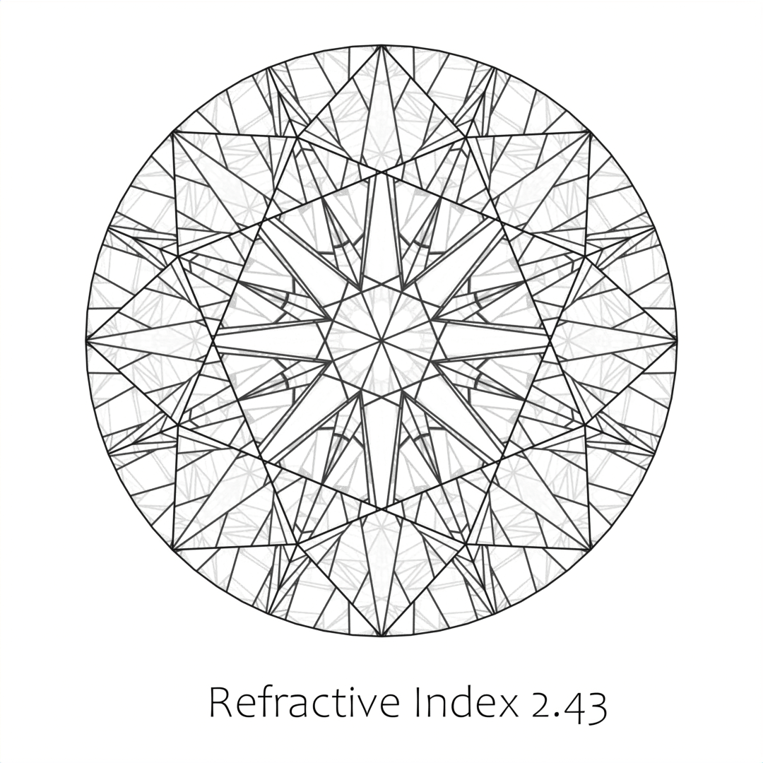
Notice that virtual facets which are right next to each other to an observer draw light from very different locations.(In crushed ice regions, the scrambling is even more severe.) Diamonds are light-scrambling sculptures! This light-scrambling property of faceted diamonds is related to diamond’s high index of refraction, which makes total internal reflection more likely for light rays traveling within the diamond. In Figure 7 we show the virtual facet pattern for a standard round brilliant cut from materials with different refractive indices.
The analysis illustrated in Figure 6 is the core of an algorithm called beam tracing, in which one models a beam of light as parallel rays interacting with the diamond, subdividing the beam into smaller beams as it encounters different facets (beamtrace?). Beam tracing is an exact algorithm if the eye is assumed to be at infinity (orthographic) so that the rays are all parallel, but is still a reasonable approximation at the usual viewing distances of diamonds. In this paper, both orthographic beam tracing and perspective ray tracing are used.
(CutGroup?) argue that for a full understanding of diamond visual perception, one needs to incorporate binocular vision. The authors say that maximum brilliancy occurs when a virtual facet appears illuminated to one eye while dark to the other, which is related to the phenomenon of binocular luster (luster?). We do not further pursue this fascinating hypothesis in this paper, but note that it does bring up the important point that each eye will see a slightly different virtual facet pattern.
3. MODELING THE RELEVANT OPTICAL DETAILS
In the previous section we described how a beam of light traced back from the eye fragments into polygonal beams that draw light from different locations surrounding the diamond. This is a simplification of what actually happens because it ignores beam splitting at material interfaces. We discuss some of that subtlety here.
Like most interactions of light with a transparent medium, a light ray entering a diamond from the outside splits into two child rays. The one that reflects off the facet is called specular reflection (or more informally glare), and the other ray which penetrates into the diamond, refracting according to Snell’s law, is called the transmitted ray. Once inside the diamond, those rays that meet a facet at an angle far enough from perpendicular are forced to reflect off the facet internally and cannot exit the diamond (Total Internal Reflection). However, when an internal ray meets a facet between perpendicular and the critical angle, generally it splits into two rays, and again one child ray reflects back into the diamond, and the other exits the diamond. The child ray that exits the diamond is called the primary ray while the child ray that reflects back into the diamond is called a secondary Fresnel reflection. The primary ray approximation neglects specular reflection and traces only primary rays.
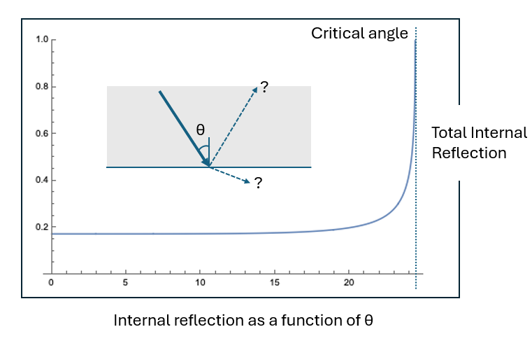
The fraction of energy carried by an exiting ray is remarkably close to a step function, typically carrying a little more than  of the ray’s power, unless the angle happens to be extremely close to the critical angle. This is illustrated for light at
 nm in Figure 8, with a 2D contour plot for other wavelengths in Figure 9. The amount of power carried by the internally reflected ray is graphed as a function of incident angle. It remains fairly level at a little over
 of the original ray strength, until it shoots up to 100% at the critical angle. These graphs were calculated using Fresnel equations for light of randomly mixed polarization. (See the note on polarization in Section 3.1.) The critical angle which forces internal reflection can be calculated as
 for index of refraction
 .
One thing we see from the graphs in Figures 8 and 9 is that sufficiently close to the critical angle, more energy is carried by the reflected ray than by the transmitted, refracted ray. We call the break-even point where equal energy is carried by both child rays the modified critical angle. We are introducing this angle here as a potential substitute for the critical angle when calculating primary ray paths. In this framework, the primary ray would be the one that carries the most energy.
We calculated both critical angles and modified critical angles in Table 1 for a range of wavelengths to understand the difference between the two potential definitions of primary ray. The difference between the critical angle and the modified critical angle is on the order of  , which is less significant than the difference coming from different wavelengths, lending support to the accuracy of the standard primary ray approximation.
Critical angles vs modified critical angles. The modified critical angle is the threshold at which reflected and transmitted light carries equal power.
| Wavelength (nm) | Refr. index | Crit. angle (°) | Mod. crit. angle (°) |
| 400 | 2.458 | 24.01 | 23.77 |
| 450 | 2.443 | 24.16 | 23.92 |
| 500 | 2.429 | 24.31 | 24.07 |
| 550 | 2.421 | 24.40 | 24.15 |
| 600 | 2.414 | 24.47 | 24.23 |
| 650 | 2.410 | 24.52 | 24.27 |
| 700 | 2.406 | 24.56 | 24.31 |
| 750 | 2.401 | 24.61 | 24.37 |
| 800 | 2.400 | 24.60 | 24.38 |
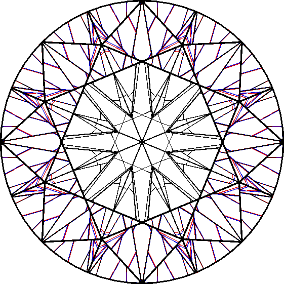
The higher order reflections (which carry a small percentage of the energy) are faintly visible in the lefthand image of Figure 10.
Tracing a ray from the eye back into the diamond gives rise to a tree of rays. When it hits the diamond, it splits into a glare component and the component entering the diamond. Every time it hits a facet outside the critical angle, a component typically carrying over of the energy exits the diamond to find a light source in the external environment. Thus what we see is actually a superposition of primary rays, secondary rays, tertiary and so forth.
In a diffuse lighting environment, because the primary rays carry much more energy than the secondary and tertiary rays, it is often safe to ignore the contribution of the higher order rays. They have a minimal impact on modeling the relative amounts of energy that return through the crown or exit away from the observer. However, in a spot light environment, the secondary and tertiary rays do have a noticeable impact. This is because a light source may be positioned in a location from where a secondary virtual facet collects light, but there is no light source positioned where the corresponding primary virtual facet collects light. As a result, the observer sees an illuminated secondary facet, significantly dimmer than the light source, but still much brighter than neighboring (secondary) virtual facets.
(refract?) derive an equation for refractive index,  , as a function of wavelength,
 , that best fits the measured data:
This is a simplified version of a Sellmeier equation, which fits the data within measurement error just as well as those with more terms. This simplified formula was used to create the contour plot in Figure 9.
The refractive index varies from n=2.4709 at 380nm to n=2.3994 at 780nm. This means that there is a slightly different virtual facet pattern for each frequency of light, as illustrated on the right of Figure 10 for a standard round brilliant. In some cases, if a beam of light reflecting within the diamond hits a facet at close to the critical angle, part of the spectrum may undergo total internal reflection, while the rest of the spectrum may partially refract out of the diamond.
Indeed, it is not unusual for a round brilliant with a steeply cut pavilion to have brownish virtual facets around the inner edge of the table, due to the fact that the light paths for the blue end of the spectrum end up coming from below the diamond, while the red end of the spectrum has light paths which come from above the diamond at an angle that can find a light source. This phenomenon, known as partial leakage, was pointed out to the first author by Janak Mistry (Janak?). The reason the color is rusty brown and not a more saturated spectral color is the continuous interpolation between the frequencies that follow one path or the other in the Fresnel equations. If the reflectance graph were a true step function, we would expect the colors to be more saturated. Computer simulations confirm this analysis.
3.1 NOTE ON POLARIZATION
According to Fresnel’s equations, differences in the reflectance for different polarizations at each facet interaction will change the polarization mix of the light. In practice, including polarization in ray tracing calculations tends not to change the result significantly. It doesn’t affect the primary ray trace at all, but may subtly affect the intensity of secondary reflections, especially as seen through non-table facets. We calculated the difference in intensity of an example primary ray in a cross section of the standard round brilliant and found a difference of about  percent. Moreover, for complex light paths, shifts in reference frame will tend to destroy any cumulative partial polarization effects. One possible exception that deserves further study is an emerald cut where many ray paths are close to planar.
3.2 THE IMPORTANCE OF SECONDARY RAYS
For a diffuse lighting environment, the primary ray approximation is often sufficient to get a qualitative sense of diamond performance. Secondary virtual facets are washed out by the more powerful primary virtual facets, and contribute little to the overall assessment. However, one diffuse-light situation where considering secondary rays has proved useful is in evaluating windowing or leakage. See Section 5.1.
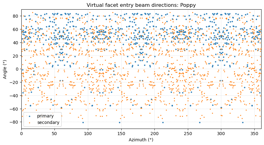
In a spot lighting environment, secondary virtual facets become much more important. This is because sparse light sources that illuminate a secondary, or even tertiary virtual facet, may not have any competing light sources positioned to illuminate the corresponding primary virtual facet that would normally wash it out. Moreover, the secondary and tertiary facets can exhibit more fire because they correspond to longer ray path lengths, giving more opportunity for dispersion. See Figure 11. The secondary virtual facets tend to dominate in very sparse lighting environments because they collect light from a larger set of directions than the primary virtual facets. In fact, in a certain sense, the secondary virtual facets dominate in very sparse lighting environments because they collect light from a strictly larger set of directions than the primary virtual facets. See Figure 12.
In one experiment, a subset of the authors observed several fancy cut diamonds in direct sunlight. The sun’s angular diameter is approximately 〖0.5〗^∘, so qualifies as a spot light source. In each case, most of the diamond appeared dark because the majority of virtual facet light source directions did not overlap with the sun’s position. Virtual facets that directly reflected the sunlight back to the eye were blindingly bright. Avoiding holding the stone at those angles where primary virtual facets reflected the sun, there was a spray of smaller dimmer colored sparkles across the stone’s surface which represented both secondary and tertiary virtual facets.
4. COMBINATORIAL DESCRIPTION OF VIRTUAL FACETS
Tracking each (primary) ray back from the eye, we get a list of facets it interacts with. First it enters the diamond along some facet, then in general sequentially reflects off of several facets from the interior of the diamond, and then exits via some facet. We claim that for a convex diamond, every virtual facet is uniquely identified by this list of facet interactions. Or to put it another way, if we define a virtual facet to be the set of rays that have the same ordered facet interaction list, they form a convex (in particular connected) polygon. Actually there is one potential exception when there are facet interactions near the critical angle, though this exception is not present if we use orthographic tracing—i.e., if we assume the observer is at infinity and the light being reverse traced from the eye is collimated. Let us now formalize this discussion.
Definition 1. Let  be a polyhedron with some fixed index of refraction
 within a medium with index of refraction equal to
 . A primary ray starts outside of , with its trajectory determined by the following rules:
- When it encounters a facet from the exterior of
 , it continues into with direction altered according to Snell’s law
 , where
 is the angle of the incident ray with the normal vector and
 is the angle of the transmitted ray from normal.
- When the ray hits a facet from the interior of , if the angle with the normal direction exceeds the critical angle of
 , the ray reflects off the facet according to the rule that the angle of incidence equals the angle of reflection.
- If the ray hits an internal facet within the critical angle, it transmits out of the diamond, again according to Snell’s Law.
- Supposing the previous definitions, every virtual facet, viewed as a subset of the viewing plane, is convex, hence connected.
- The boundaries of virtual facets represent ray paths that intersect the
 -dimensional edges of the polyhedron.
We assume the ray path is generic in the sense that it never meets facet boundaries.
Definition 2. Consider collimated (parallel) light rays traced through a convex polyhedron , using the rules governing primary rays from Definition 1, with some fixed index of refraction , within a medium of refractive index . A virtual facet is defined as the set of rays which have a specified facet interaction sequence. One may regard the virtual facet as a subset of the viewing plane, which is a plane orthogonal to the light direction that intersects the light rays before they meet .
Theorem 1.
Proof. Consider a list of facet interactions  , and assume that at least one light path has this facet interaction sequence. If not, we have a degenerate empty virtual facet.
The first facet  is the entry facet into the diamond. So we truncate the beam so that it just passes through the facet . The facet is convex since it is a facet of a convex polyhedron. Consider the set of light paths meeting , and truncated to stop at . These form an oblique polygonal cylinder, infinite in one direction, with base . The rays in the beam will still follow different directions (sub-beams) after leaving . See Figure 6 for an illustration, which shows a beam intersecting a single crown facet , but then splitting up into multiple sub-beams in subsequent stages.
The segment of the beam consisting of light paths from into the diamond begins to sweep out another oblique convex polygonal cylinder by displacing along the direction of refraction. Hence the set of all light paths from to  is determined by the intersection of this cylinder with the convex facet . In other words the set of points on that are reached by
 light-paths is a convex polygonal subset
 .
Next, if the truncated beam meets inside the critical angle, it will transmit out of the diamond and no further facet interactions would be possible, implying was the last facet in the list and  . Otherwise, the beam reflects back into the diamond, geometrically being represented by displacing
 along the reflection direction, sweeping out an oblique convex polygonal cylinder, which then intersects with
 in the convex sub-polygon
 .
Continuing this analysis, each time we are taking the intersection of a convex beam segment with a convex facet, so the resulting facet intersections are always convex. It might be helpful to consult Figure 15, which shows two totally trimmed beams corresponding to unique virtual facets.
As we trim down the beam, the light paths on the boundary of the beam are always coming from intersections with facet boundaries. To see this, note that the virtual facet comes from an iterative trimming process, which starts with the polygon , then is formed by intersecting a translation of with . So all edges of are either translates of subsets of edges of or subsets of edges of . Similarly at each stage  is the intersection of a translation of
 along the beam direction with
 , so all edges come from facet edges. This establishes the second claim of the theorem. ◻
The second result in the the above theorem implies that the visual field, when looking at a diamond, is subdivided into small polygons by the reflected and refracted images of the -dimensional edges of the diamond itself, and the interiors of these polygons represent similar light paths through the diamond, which is what we call virtual facets.
In the case of perspective ray tracing, as opposed to orthographic beam tracing, one may theoretically get borders between virtual facets that are not edges of the polyhedron, but are due to the fact that a bundle of diverging rays meeting an internal facet may not all have the same behavior when the test of Definition 1, condition (2) is applied. More specifically, if reverse traced rays from an observer’s eye meet a facet internally, close to the critical angle, you may have some rays that reflect and some transmit out of the diamond. This creates a border between virtual facets that is not a polyhedron edge but instead a transition coming from the Snell-derived critical angle cutoff. Such boundaries are in general curved, which means that in very rare circumstances, the region  constructed analogously to the orthographic case, where light paths reflect back into the diamond from facet , may be non-convex and non-polygonal. Further regions
 ,
 could even end up being disconnected. In practice, because we assume the eye is sufficiently far from the diamond polyhedron, the rays do tend to be very close to parallel, so the above circumstance is unusual.
5. ASET TYPE COLORINGS OF VFPS
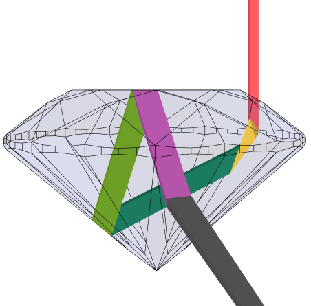
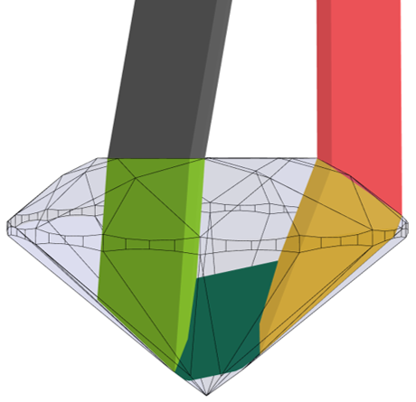
One can think of the virtual facet pattern as a template for light interaction with the environment. Each virtual facet collects light from a particular region of the external environment, and if a light source happens to be sitting there, it will appear illuminated. The class of rays within a virtual facet form a light beam, and tracing this backward out into the environment yields what we call the “entry beam” for that virtual facet. There will be slight angular variation of rays within the beam, although if one uses orthographic projection (eye at infinity) the beams are collimated.
This is often mathematically modeled by surrounding the diamond by a hemisphere and calculating the intersection of a virtual facet’s entry beam with the hemisphere. This hemisphere can be close to the diamond, or far away, which will yield different results. If one takes the limiting case of having the hemisphere at infinity, then it is only the angle the entry beam makes with the horizon that matters. The sphere at infinity can be called the celestial sphere.
Gilbertson has pioneered the idea of color coding virtual facets by the angle the entry beam makes with the horizon. Gilbertson’s original concept(Gilbertson2000?; Gilbertson2013?) is illustrated on the left of Figure 13. The exact cutoffs are given in Table 3(a).
Colorings by entry beam angle. Left: ALGW, Right: ASET
| Entry beam angle (°) | VF color |
| Black |
| Red |
| Green |
| Purple |
| Light blue |
| White |
 –
 (near vertical)
 –
 –
 –
 –
 (below horizon)
Colorings by entry beam angle. Left: ALGW, Right: ASET
Entry beam angle (°) | VF color |
| Blue |
| Red |
| Green |
| Grey or White |
 –
 –
The software DiamCalc by OctoNus(diamcalc?) refers to this map as an “Al Gilbertson Map.” We refer to it as the ALGW map, the “W” indicating that the environment below the diamond is white.
AGS Lab introduced a simplification of the Gilbertson map, called the ASET map (AGS?), which stands for “Angular Spectrum Evaluation Tool” (See Table 3(b) and Figure 13 middle.)
When one looks directly at a diamond, the entry beams that are close to vertical will tend to originate from the observer’s upper body and head. The corresponding virtual facets will appear dark, because the observer is much less luminous than the surrounding environment. The terms obscuration and “head shadow” have been used to describe this effect, but it occurs in the same manner whether the primary light source is behind or in front of the observer. Entry beams from mid-range angles sample the bright parts of the environment around the observer, and tend to produce bright virtual facets. Shallow entry beams sample dimmer areas and tend to yield dull virtual facets. Thus, VF patterns colored by their entry angle range summarize the relative light return for a given diamond geometry.
While the ASET is simpler and easier to understand, it captures less information than the ALGW map. However in some cases that simplicity reveals relevant features that are more subtly expressed in the ALGW coloring. For both maps, the color chosen for the area below the diamond reveals windowing (leakage) from rays that pass through the diamond without internal reflection. In the maps shown throughout this paper, this background color is white or grey depending on the software used to produce it.
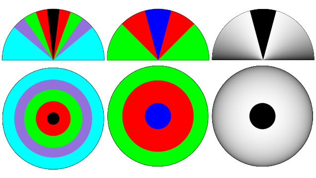
The ALGW map has 5 colors encoding the upper hemisphere, while the ASET only has three. Another possible simplification is to use a continuous grey scale from  to
 . Such an encoding is pictured in Figure 13. This so-called “mono” ASET models diffuse lighting with obscuration. Angles from to
 are colored black, while angles outside that region are colored using the cosine of the angle with the vertical, with brighter light corresponding to higher angles. A cosine light distribution is a standard model for overhead light. In addition to a cosine weighting, cosine squared has been used previously by GIA researchers as an illumination model without head obscuration (hemphill98?) and as a measure of significance of chromatic flares (Fire2001?).
One disadvantage of both the classic ASET and ALGW map is the presence of discontinuous cutoffs. A stone which has been scanned twice might have discrepancies in VF color due to minor measurement differences. This is a persistent phenomenon in one popular geometry for round brilliants, as the central virtual facets (often called table reflection virtual facets) correspond to light entering the diamond at a  angle, which is right at the boundary between the red and the green zones. This issue is mitigated though not absent in the mono ASET. Taking into account a range of tilts when tracing ASETs and forming a holistic assessment from the set of tilts also offsets the problems raised by discontinuous cutoffs.
Refer to Figure 14 for different versions of the ASET of the standard round brilliant. The associated beam paths for two virtual facets are shown in Figure 15.
The ASET map has become a widely used method for evaluating diamond performance within the industry, in part due to AGS Lab’s popularization of it.
5.1 DUAL ASETS
The computer modeled ASETS described in the previous section only take into account primary rays. A dual ASET is an ASET in which an ASET coming from the primary ray approximation is blended with an ASET traced using secondary rays, with relative brightnesses computed using the appropriate Fresnel equations. In Figure 16, we have pictured both primary and dual ASET for one of our research pear-shaped diamonds, with leakage/windowing in white. One can see that the windowing in the head is ameliorated by the secondary reflections, a fact confirmed through direct observation.
Dual versions of the the ALGW and Mono ASET maps are also useful.
A (primary) ASET map (Left) and dual ASET map (Right) for a pear in our research collection. Although the primary ASET indicates large dead areas in the head due to windowing, the dual ASET shows that these areas are broken up by secondary illumination.
5.2 VIRTUAL FACET INFLUENCE
In the standard round brilliant diamond, most virtual facets are roughly the same size and apparent distance from the eye, so the overall pattern is perceived clearly. However, for many fancy shapes, there are a few prominent virtual facets, the ones that are bigger and tend to have shorter light path lengths, surrounded by less distinct, fuzzier and smaller, virtual facets. In order to capture this, we have created a visual influence score (VI) for each virtual facet, that measures how significant a virtual facet is to an observer.
Definition 3. Let  be a virtual facet regarded as a subset of the viewing plane. Define the visual influence score by the formula
where  is the face-up area of the virtual facet, measured as a fraction of the entire diamond’s footprint area,
 is the length-to-width ratio of an oriented bounding box, and
 is the average ray length of the corresponding beam of light inside the diamond, measured in millimeters.
This value is used as an ingredient in various Visual Performance metrics. For example, we can enhance one classic measure of diamond brightness as follows. The classic AGS Lab system used the relative area of red in the ASET diagram as a brightness measure. This can be conceptualized as
where  is the indicator function which equals if and only if a virtual facet is colored red in the ASET map. This can be modified to give a new type of brightness score:
The resulting quantity is scale-invariant: scaling the diamond by a constant factor  will introduce a factor of into each , which will cancel in the quotient.
Along these lines, in Figure 17, the colors of a standard ASET are given brightnesses calculated from the virtual facet influence scores, so that the virtual facets contributing the most to the diamond’s appearance are brighter.
The idea is that the illumination status of high influence virtual facets is more significant than that of lower influence virtual facets. Clearly the bigger the VF is, the more noticeable, which is why is included. Less clearly, we claim that the less oblong and more compact a VF is, the more important it is perceptually, explaining the term, and finally the closer the VF appears to the eye (the shorter the light path), the more important it is. Longer light paths may mean the VFs are harder to keep in focus, and also account for light absorption. We are assuming our diamonds are nearly colorless, but even in that case, there is some dimming along longer light paths.
For example, a high-VI virtual facet that exhibits windowing will have a more deleterious effect on the diamond’s appearance than a set of smaller leaky virtual facets that add up to the same area. In addition, these influential portions of the VF patterns tend to persist across changes in viewing angle because of the shorter path lengths.
When testing competing metrics against observations, we have found that metrics incorporating visual influence consistently outperform alternative metrics.
6. VIRTUAL FACET PATTERNS AND FOCAL DISTANCE
Every virtual facet corresponds to a string of facet interactions. Since there are always the entry and exit facets, we call a virtual facet with  facet interactions a -flector, corresponding to the internal reflections. This gives an alternative method to path length—previously mentioned as a fundamental ingredient in the visual influence score (Section 5.2)—for measuring light path complexity.
A  -flector is a virtual facet where the light traced back from the eye enters the crown and then exits the diamond somewhere, typically through the pavilion. This is an example of windowing where you can see through the diamond.
A -flector will correspond to reverse-traced light entering the crown, reflecting off a single pavilion facet, and then exiting the diamond somewhere. Based on the geometry, it could exit via the pavilion, girdle, or crown.
The vast majority of the surface area of a standard round brilliant is composed of  -flectors, where the light enters the crown, reflects twice off the pavilion, and then exits the crown. For fancy shapes, the light ray paths can get a lot more complex, and you can have
 -flectors and beyond. See Figure 18 for a comparison of standard round and oval.
This actually leads to an interesting mathematical question.
Conjecture 1. There are polyhedra, refractive indices, and viewing positions for which there are -flectors with arbitrarily large within the same VF diagram.
There is evidence that this is true for diamond’s refractive index of  , but it may be easier to prove for a larger refractive index, which will make it less probable that a primary ray will meet a facet within the critical angle.
It seems conceivable, and some experimental evidence points in this direction, that in stones with crushed ice, the set of -flectors of increasing limit onto a Cantor set. Plots set at the highest resolution have found  -flectors. The chaotic light paths found in -flectors of large is reminiscent of chaotic billiard path dynamics, except in the case of diamond light paths, the “billiard ball” has an escape condition forcing it to exit the polyhedron if it meets a face sufficiently close to normal. (See Definition 1.)
The path length of -flectors will tend to get longer as increases. Scatter plots of average path lengths of virtual facets for pear and oval are given in Figure 19. Size of a virtual facet is an inversely correlated variable to both path length and .
Virtual facets that correspond to long light ray paths will appear further away, and tend to be out of focus. These virtual facets tend to be small and part of what is known as “crushed ice.” This is common in fancy shapes. We invite the reader to try focusing their eyes at a distance next time they look at a fancy diamond, and they may find that different features of the apparent internal structure of the diamond come into focus. See Figures 20 which show how different virtual facets come into view at different focal depths. This phenomenon is very apparent for diamonds viewed with a loupe.
If one has the opportunity to observe very large diamonds (e.g. over  carats), the virtual facet pattern has an apparent three dimensionality to it, almost like soap film moving around within the diamond’s interior.
As mentioned in Section 5.2 the lower depth virtual facets tend to be quite noticeable to the eye, whereas the deeper and smaller virtual facets may not be in focus and do not necessarily correspond to what is observed. Qualitatively, a region of ray-traced crushed ice is correct, but the various physical and mathematical approximations and 3D model scan fidelity limitations are compounded on long ray paths, leading to a loss of fine scale visual fidelity. One reason the model quality remains good, however, is that crushed ice regions tend to draw light from a random set of directions, distributed evenly over the surrounding sphere.
7. DIFFUSE LIGHTING FEATURES OF VIRTUAL FACET PATTERNS
For the diffuse environment, we adopt a mathematical model based on the mono ASET described above. It uses a dark spot at the north pole of the celestial sphere, subtending a  angle to simulate obscuration, with a light source positioned above the stone following a cosine power distribution. Tracing light from this environment through a modeled geometry produces a map that encodes the likelihood that portions of the VF pattern will appear dark because they only gather light from obscured directions.
In this section we look at various features of virtual facet patterns of diamonds that occur in a diffuse lighting environment. We start by discussing the “arrows” pattern in a standard round brilliant and some other shapes, and transition to “bow-tie,” which is caused by the same optical phenomenon. We also discuss crushed ice and girdle reflection.
7.1 Hearts and arrows
At one point in time, standard round brilliant diamonds formed the vast majority of diamonds graded by GIA, but it would be an understatement to say fancy shapes are increasing in popularity. One of the most well-known virtual facet patterns, formed by dark virtual facets, is the “arrows” side of the “hearts and arrows” pattern.(The “hearts” side of the pattern is visible when viewing the pavilion.) The arrows are seen clearly in Figure 1: eight dark symmetrically arranged “arrow shafts” are seen in the table, with dark grey “arrow heads” seen in the bezel facets. These are well-captured in the ASET map in Figure 14 as well. Many consumers and retailers appreciate this patterning of a round brilliant diamond. Some other shapes can also have hearts and arrows type patterning, including various cushion cuts.
7.2 BOW-TIE
If one takes a standard round brilliant and alter the length-to-width ratio, one gets a type of oval cut where the pavilion mains remain aligned with the crown bezels. (See Figure 3 for definitions.) The two arrows of the virtual facet pattern which are perpendicular to the axis of elongation (i.e. at the belly) tend not to change too much, and so many oval cuts have a dark band across their belly, often called bow-tie.
The darkness of the virtual facets creating the bow tie and arrows pattern is caused by head obscuration. In other words, the direction from which the virtual facet is collecting light is in the direction of the observer’s head, which is not a light source. In photos, these virtual facets pick up the color of the camera.
Bow-tie also occurs in marquise and pear cuts (Figures 20 and 21.) Note that Figure 21 uses an obscuration map in addition to the classic ASET. The obscuration map colors facets darker the more persistent the obscuration and can be thought of as a discrete version of the Mono ASET map that doesn’t encode leakage at all. Pears and marquises with bow-tie tend to have a band of large virtual facets across their belly, with regions of crushed ice to either side. As with oval shapes, some of these large virtual facets tend to appear dark.
Unlike in the round brilliant, there is a tendency to want to minimize bow-tie in fancy shapes, which has led manufacturers to cut shallower pavilion main angles, and even to switch to a different pavilion facet arrangement where the pavilion mains are not aligned with the crown bezels (Janak?). (Figure 26 shows an  -main oval where the crown bezels are aligned with the pavilion mains. There is an alternative faceting arrangement where the pavilion mains point halfway between the crown bezels.) Examples of pear- and oval-shaped diamonds without bow-tie can be found in Figures 22 and 23.
A study of bow-tie dependence on angle variations in a 7-main pear is depicted in Figure 24. Crown and pavilion angles (at the stone’s belly) were varied, while keeping other measurements as constant as possible, and the resulting contrast maps are displayed. Considerable variation in bow-tie patterns is found across this range of angle variations, with stronger dependence on pavilion angle. Samples with pavilion angles from  to
 show substantial bow-tie. A different study of the same facet arrangement looked at changing the length to width ratio from 1.2 to 1.8, while keeping the crown and pavilion angles fixed at
 and respectively (Figure 25). As expected, bow-tie behavior is similar in all models.
7.3 CRUSHED ICE
The term crushed ice refers to clustered virtual facets of relatively small size and is observed in many fancy shapes including ovals, pears, marquises, emeralds and cushions. Figure 26 shows common examples of VF patterns for oval and pear with crushed ice evident in both cases. Indeed, it is possible to find stone geometries that produce crushed ice for almost any facet arrangement. In general, crushed ice corresponds to light beams that have subdivided many times, and so corresponds to longer light paths. Crushed ice is a phenomenon that has mixed appeal (ggpaper?). The long ray paths lead to the optical illusion that these small virtual facets lie behind the actual diamond. With motion of the diamond, these crushed ice areas appear to flow as brightness and relative focus change rapidly.
Crushed ice generally corresponds to small virtual facets and long ray lengths, but there are exceptions. For example, if a beam encounters a girdle facet, all virtual facets formed from the child beam reflected off the girdle will have to be at least as small as that. Hence relatively low depth, but tiny, virtual facets can occur. Moreover, because of the essentially randomized nature of crushed ice, it is almost certain that virtual facets that had at least one girdle interaction will be distributed throughout the crushed ice regions.
7.4 GIRDLE REFLECTION
In some fancy shape diamond geometries, the girdle is clearly visible, reflected up into the table. For example, different views of the same girdle inscription are visible under magnification in Figure 27, and one can see other views of the girdle surrounding the culet. Even under normal viewing conditions, girdle reflections can be noticeable and distracting, especially when they are dark. Girdle reflection is an inevitable component of crushed ice regions, due to its randomized nature, but it also tends to blend in. In the worst cases, girdle reflections form prominent and distracting curvilinear dark features in the table, a pattern which is sometimes called “fisheye.”
One reason for analyzing girdle reflection, aside from assessing “fisheye,” is to predict how strongly dirt on the girdle will affect the diamond’s performance. (A similar issue has been raised by Holloway for pavilion dirt. (holloway?)) An initial guess is that girdle dirt or oil will show up in virtual facets corresponding to rays entering the diamond through the girdle on the way to your eye. To model the effect, we colored the girdle of several different fancy-cut diamonds with green marker. See Figure 28 for the case of a pear shape. The green pigment on the girdle can be seen spread throughout regions of the face-up appearance of the diamond. In the middle, we have raytraced the diamond and highlighted virtual facets in red where the rays entered the diamond through the girdle. We call this the girdle leakage map. However, it is evident that the colored girdle can be seen across a larger range than can be accounted for here. The girdle reflection map (on the right) instead highlights every virtual facet where light either entered through the girdle, or internally reflected off of a girdle facet at some point in its journey, and this distribution matches the marked diamond much better.
When we model light moving through the diamond, if the angle with a facet exceeds the critical angle, that facet acts like a mirror, so that whatever is on the other side of the facet is invisible to that ray path. However, dirt/oil on the facet with sufficient adhesion will in general alter the critical angle, because the secondary medium in Snell’s law will have been changed from air to a substance with higher refractive index. Hence it can happen that a ray that would reflect off a clean facet will actually refract through a dirty facet. So there is the possibility of seeing girdle dirt wherever a ray reflects off of a girdle facet. The phenomenon where changing the surrounding medium changes total internal reflection to allow some refraction is called frustrated total internal reflection.
The reader can see this phenomenon using a glass of water (wiki?). If you hold a glass of water loosely and observe from a certain angle, your fingers are not visible, but when you grip it tightly, the very tips—often just the fingerprint ridges—do become visible.
7.5 Returning to patterns
Large and small VFs both contribute to contrast, the interplay of light and dark elements in the VF pattern a diamond exhibits. The magnitude of light-level differences encompasses how well each virtual facet stands out from its neighbors. The distribution of light and dark elements can create a pleasingly bright appearance, or undesirable darkness. Understanding the various causes of dark VFs with respect to where they gather light from the environment can be useful for making optimal choices in executing a particular diamond design.
Diamonds without enough dark virtual facets are sometimes referred to with the disparaging term “headlights.” Too much obscuration or windowing, on the other hand, makes the diamond look dark and unappealing. Also, a dense dark region in the center of a diamond is seen as less appealing than a more distributed network of dark virtual facets. The art is to find just the right balance of light and dark areas with the highest magnitude of contrast possible. One interesting area of design innovation is the intentional usage of windowing as a patterning element similar to obscuration.
However, sometimes it comes down to personal taste. A stone that looks unappealing to one person may be attractive to another one. For example, Figure 29 depicts a photorealistic render of a fancy round diamond which many find too dark, yet others find appealing.
8. SPOT LIGHT PHENOMENA
While various pattern phenomena are best modeled in a diffuse lighting environment with an obscuration disk, both scintillation and fire are displayed more vividly under sparser spot light conditions. At first, this may seem to present a problem with quantification, given that there is no single canonical spotlight environment for evaluating a polished diamond. However, there are mathematical approaches to modeling behavior in spot light environments. Quick (jason_patent?) introduced the idea of averaging over light source placements as a way to capture scintillation potential. it is also true that the scintillation (or the rapid on-and-off firing of virtual facets as the diamond in motion encounters light sources) is correlated with virtual facet depth. Moreover, in crushed ice regions, because the light directions are effectively randomized, the dependence on light source placement is neatly avoided. When it comes to fire, we model “fire potential” for each virtual facet rather than observed fire in a particular environment.
To further illustrate how the random placement of a light source can be used to measure scintillation, recall the sphere of all light source directions, the celestial sphere. In the orthographic model, each virtual facet collects light from a single direction, corresponding to a point on this celestial sphere. On the other hand, for an observer at finite focal distance (perspective model), there is slight variation in collected light direction across the virtual facet, meaning that there is a closely clustered set of directions from which the VF draws light. This set of directions is enlarged when one includes secondary and higher virtual facets.
As an example, on the left of Figure 30, the intersection of orthographically traced primary virtual facet beams with a surrounding sphere is depicted as an equirectangular projection of the sphere. We used this as a spherical radiant map to illuminate a 3D scene and generate photorealistic renders in LuxCoreRender. The array of lights is precisely tuned to illuminate each virtual facet.
8.1 SPARKLE PROBABILITY
Now imagine putting a light source of fixed angular radius  randomly in the sphere, say in the red ASET zone, between
 and from vertical. If the light source happens to intersect with the set of VF directions, the corresponding virtual facets will be illuminated. We define sparkle probability to be the probability that a light source illuminates at least one primary or secondary virtual facet. In order to model sunlight scintillation, tertiary VFs can also be included.
From a mathematical perspective, this probability can be calculated as the area of the set of all points on the sphere between and from vertical that are distance  from a VF direction, divided by the area of the set of all points in this angular range.
The sparkle probability can be calculated for a face-up or tilted view of a diamond, and measures the probability that the diamond has at least one sparkle, given a randomly placed light source in the ASET red zone of the celestial sphere.
In addition to calculating a numerical value, we can visualize the celestial sparkle map: we color in every point of the celestial sphere where a light source will illuminate at least one virtual facet. In Figure 12 an equirectangular projection of the celestial sphere is shown, with virtual facet light source directions depicted for both primary and secondary virtual facets. (The diagram at the bottom of Figure 30 is similar, but only for primary rays, and with VFs slightly thickened.) The sparkle probability can be interpreted as the probability that a randomly placed light source in the to band will intersect at least one of the pictured dots.
8.2 SPARKLE AREA AND ILLUMINATION BIAS
One issue with sparkle probability is that it doesn’t account for the size, number, or spatial distribution of sparkles. To measure these, we introduce two metrics (and corresponding celestial maps): sparkle area, and sparkle spread. Sparkle area is the average area of illuminated virtual facets for a randomly placed light source of radius in the ASET red zone, and can be calculated numerically in a manner similar to sparkle probability. The corresponding sparkle area map colors the celestial sphere using a color gradient to represent illuminated area for each light collection direction.
Finally we have sparkle spread, which measures the average spatial distribution of illuminated virtual facets. As a quick and easy way to measure this spatial distribution, we take the area of the convex hull of the illuminated virtual facets as a fraction of the total area of the visible diamond. The sparkle spread metric is then defined to be the average value of this function on the to band of the celestial sphere.
We were led to define the sparkle spread metric after we had the Sunray diamond cut, and noticed a marked asymmetry of darkness in the table when it was held next to a wall. The round brilliant and Sunray are compared in Figure 31. Figure 32 depicts the sparkle spread metric in the to from vertical range. The lighter the color, the more dispersed the illuminated virtual facets are when a light source is placed at that point.
8.3 FIRE
As we saw earlier, different wavelengths of light correspond to different refractive indices for diamond, causing a beam of white light to become spatially dispersed as it travels through the diamond toward an observer’s eye. Such dispersion leads to the appearance of prismatic color in a diamond, a phenomenon called fire. A basic measure of fire potential for a fixed virtual facet would be to measure the distance between the endpoints of two rays of different wavelengths starting at a particular point in the environment. This is called forward dispersion. One can similarly define reverse dispersion by tracing rays backwards from the eye out into the environment. These actually give different answers (AGS?), a phenomenon labeled anamorphic magnification in the referenced paper. As a beam of light travels through the diamond, its cross-section changes shape, either compressing or widening in an asymmetric way, which gives an overall directionality to calculations of dispersion.
Forward dispersion has the most straightforward interpretation. As a beam of light spatially disperses, it creates a “chromatic flare.” The more spread apart the flare, the easier it would be for it to be partially clipped by an observer’s iris, leading to perceived color. However, reverse dispersion also has a physical interpretation. Think of a “virtual chromatic flare” as the result of a reverse ray trace of a set of collinear rays at different wavelengths. This forms the set of ray paths that lead to a particular ray emanating from the diamond toward the eye. If all such ray paths hit a light source, then the wavelengths combine to form white light. However, if this virtual chromatic flare only partially intersects a light source, then only a subset of wavelengths reach the eye, leading to the perception of color in that direction. More subtly, differences in illumination intensity across the reverse traced chromatic flare footprint yield a different mix of light wavelengths than the ambient illumination, which leads to fire which is less saturated than if there are sharp cutoffs in illumination.
We found that there is a very tight linear correlation between reverse and forward dispersion for the 180 fancy-shaped diamonds in our research collection: forward dispersion tends to be about 85 percent of reverse dispersion (Figure 33).
Interestingly, we found that a linear combination of forward and reverse dispersion for a range of tilts has the most correlation with human observation. Details, as well as other approaches to fire, will appear in a future paper.
9. NEW DIAMOND CUTS
(match?) introduced a mathematical algorithm to enumerate all possible diamond crown and pavilion faceting arrangements with at least three fold symmetries. Using the output of this algorithm, our team at GIA (Jessica Jacobitz, Natalie Maddy, Kathryn Overton, and Elizabeth Polk) selected dozens of interesting faceting arrangements. 3D models were then created and their light performance was optimized.
A prototype cut grade metric was used as the objective function in a COBYLA optimizer (cobyla?) with multiple random starting points to find a set of stone parameters with the highest prototype cut grade. The COBYLA algorithm was chosen because it does not need gradient information to work. The objective function requires a ray or beam trace, which is very fast for shapes with low depth virtual facets, but can take several seconds for fancy shapes depending on resolution and degree of parallelization.
After optimized models were found for each facet arrangement, photorealistic video renders were created using Cutwise software (cutwise?). The team looked through the renders and picked a handful that looked the most interesting. Some of these were further refined. We created ALGW grids for the stones, varying crown angle, pavilion angle, and table size, and Gilbertson himself selected the models that in his experience would be the most visually appealing. We submitted some of the top models to a diamond manufacturer in Surat, India for cutting.
The octagonal Jasmine Cut was already shown in Figure 4. It has a nice even distribution of virtual facet sizes. Figure 34 depicts three other new cuts. The hexagonal poppy also has an even distribution of virtual facets as well as a pleasing alternating pattern of light and dark VFs. The Sunray’s virtual facet pattern matches its names with many radial virtual facets emanating from the center. This particular version of the Sunray has very high fire, something every observer who has seen it has remarked upon. (There is another version of the cut that emphasizes a more traditional round brilliant style contrast pattern.) The Blossom is quite interesting. The virtual facets away from the table are denser and have more brightness and color variation than the ones within the table region. All these cuts have minimal variation in facet depth, and are more similar in design aesthetic to a standard round brilliant than to oblong fancy shapes with crushed ice.
Indeed, for shapes with this much symmetry, crushed ice does not really play a role, but rather brightness, windowing, fire, and dynamic contrast are the main components of appearance. Figure 35 contains two kinds of brightness maps for differing tilts, with the standard round brilliant given as a basis for comparison.
The poppy and round brilliant have the most face-up and dynamic contrast, with the poppy even incorporating some windowing as a design feature. The poppy does have more severe windowing at a tilt. The overall brightness is similar among all stones, though for these proportions, the Sunray has fewer and more scattered contrast elements. The blossom holds its pattern stably under tilts.
Although it is not evident from these maps, calculations show that the Sunray has the most fire potential, barely edging out the round brilliant. On the other hand the poppy has relatively low fire potential compared to the other three stones, but it really stands out in terms of dynamic contrast.
In addition to experimenting with shapes that have fold symmetries, the team has created some rotationally symmetric diamond models using our own custom software. For example, Figure 36 shows a photorealistic render of a diamond with a pinwheel pattern in the center.
In future work we plan to systematically explore the space of oblong designs.
We thank Michael Cowing, Janak Mistry, Siddhant Shah, and Sergey Sivovolenko for stimulating discussions and for sharing their knowledge and expertise. We thank Robert Bryson and the anonymous referees for a careful reading of this paper and editorial suggestions. All authors gratefully acknowledge the support of the Gemological Institute of America, which funded this research.
Conant, J. (2024). Enumerating diamond cuts. MATCH Communications in Mathematical and in Computer Chemistry, 91(3), 593–631.
Cowing, M. (2009, April). The Central Ideal. Gems and Jewellery, Vol. 18, No. 2.
Cutwise Software. Lexus OctoNus, cutwise.com.
Diamond Calculator (DiamCalc) Software. Lexus Octonus.
Dodson, J.S. (1979). The statistical brilliance, sparkliness and fire of the round brilliant-cut diamond. Diamond Research, pp. 13–17.
Gilbertson, A. (2000). Device for judging symmetry, brightness, and efficacy of light return in precious stones. U.S. Patent 6665058, filed May 24, 2000, issued Dec. 16, 2003.
Gilbertson, A. (2013). Optimizing face-up appearance in colored gemstone faceting. Gems & Gemology, Vol. 49, No. 2, pp. 64–81.
Harding, B.L. (1975, Fall). Faceting Limits. Gems and Gemology, Gemological Institute of America.
Hemphill, T.S., Reinitz, I.M., Johnson, M.L., Shigley, J.E. (1998, Fall). Modeling the appearance of the round brilliant cut diamond: an analysis of brilliance. Gems and Gemology, Gemological Institute of America.
Holloway, G. (2024). How to Select the Best Diamonds: Insider Secrets. Self-published. Available at: https://www.amazon.com/How-Select-Best-DIAMONDS-Insider/dp/0645801410.
Kato, M. (1982, June). Re-examination of optimum cutting angles between main facets of gemstones based on geometrical optics. Summarized Translation of Journal of the Gemmological Society of Japan, Vol.9, No.1, 3–17
Liddicoat, R. T. (1993) The GIA Diamond Dictionary. United States: Gemological Institute of America.
LuxCoreRender Team. LuxCoreRender. https://www.luxcorerender.org.
Mistry, J. (2023). personal communication.
OctoNus. Publications https://www.octonus.com/publications
Powell, M. (1994). A Direct Search Optimization Method That Models the Objective and Constraint Functions by Linear Interpolation. S. Gomez and I-P. Hennart (eds.) Advances in Optimization and Numerical Analysis, 51-67. Kluwer Academic Publishers.
Quick, J. (2013) Systems and methods to measure and display the scintillation potential of a diamond or other gemstone. U.S. Patent 9599570, filed October 10, 2013, issued March 21, 2017
Reinitz, I.M., Johnson, M.L., Hemphill, T.S., Gilbertson, A.M., Geurts, R.H., Shigley, J.E. (2001, Fall). Modeling the appearance of the round brilliant diamond cut: an analysis of fire, and more about brilliance. Gems and Gemology, Gemological Institute of America.
Reinitz, I.M., Gilbertson, A., Blodgett, T., Hawkes, A., Conant, J., Prabhu, A. (2024, Fall). Observations of Oval-, Pear-, and Marquise-Shaped Diamonds: Implications for Fancy Cut Grading. Feature Gems & Gemology, Vol. 60, No. 3, Gemological Institute of America.
Sasian, J., Quick, J., Sheffield, J., Caudill, J., Yantzer, P. (2007). Evaluation of brilliance, fire, and scintillation in round brilliant gemstones. Optical Engineering, 46 (9), Article no. 093604.
Sivovolenko, S., Shelementiev, Y., Holloway, G., Mistry, J., Serov, R., Zhulin, S, Zipa, K. (2013). How diamond performance attributes: Brilliance, Scintillation and Fire depend on human vision features. The Australian Gemmologist 25 No.3 82-121.
Tolkowsky, M. (1919). Diamond Design, Spon and Chamberlain, New York
Turri, G., Webster, S., Chen, Y., Wickham, B., Bennett, A., Bass, M. (2017). Index of refraction from the near-ultraviolet to the near-infrared from a single crystal microwave-assisted CVD diamond. Optical Materials Express 855, Vol 7, No 3
Voelker, M., Hamann, B. (2007). Real-time rendering of cut diamonds. technical report, Dept. Of Computer Science, UC Davis
Wendt, G., Faul, F. (2022) Binocular luster – A review. Vision Research, Volume 194, 108008, ISSN 0042-6989
Whitlock, H.P. (1917, May 9). The Proportions of the Brilliant Cut. The Jewelers’ Circular-Weekly
Wikipedia contributors. (2025, August 9). Total Internal Reflection. In Wikipedia. Retrieved August 9, 2025, from https://en.wikipedia.org/w/index.php?title=Total_internal_reflection&oldid=1303223713
GIA’s custom proprietary software was used to generate all images, except where otherwise noted. ChatGPT and Microsoft Copilot were used for help in formatting the LaTeX source code for this document, as well as formatting help in the production of Python figures (Figures 6, 9, 15, 33). The actual data content was supplied by GIA’s custom ray and beam tracing software. The image of a person in Figure 6 was created by ChatGPT.
Conant
ABSTRACT
Diamonds used in jewellery represent the quintessential fusion of aesthetic appeal and technical expertise. Not only does it require extreme skill to cut a diamond, analyzing and predicting a diamond’s Visual Performance™ is essentially a technical mathematical problem. In particular, diamonds and other faceted gems have the property that they fragment the visual field into a set of polygons called virtual facets, which represent equivalence classes of light paths according to their facet interactions with the gem polyhedron.
In this paper we explain how this mathematically elegant conception forms a framework from which to analyze a diamond’s appearance and beauty. We intend this framework to form the foundation for a fancy-shaped diamond cut grading system.
Although virtual facet patterning has been studied before, mostly in the context of round brilliant diamonds, a significant new feature of our approach is to take into account the effect varying visual depths of virtual facets has on visual perception. We also showcase some novel designs created by our team at GIA using a mathematical enumeration algorithm for symmetric diamond-like polyhedra.
KEYWORDS
Virtual Facet Pattern (VFP), diamond design, light performance, crushed ice, bow-tie effect, girdle reflection, scintillation, fire, fancy cut diamonds, diamond visualization, optical modeling, lighting environment, dark zoning, ASET analysis, computer simulation, diamond cut evaluation.
INTRODUCTION
Consider the diamond images in Figure 1. The geometric patterns that we see are more complex than the simple surface faceting of the diamonds, representing nontrivial light paths through the gemstone. These patterns of virtual facets (VF), also called “mosaic patterns,” represent an essential visual and aesthetic quality of diamonds. The standard round brilliant diamond typically displays a pattern with moderate-to-small sized virtual facets. Among fancy shapes (any shape which is not a standard round brilliant), some cuts display large blocky virtual facets, while others show an even distribution of very fine virtual facets. Areas of very tiny virtual facets are often called “crushed ice,” named for the similarity to the sparkles of light one might see in actual crushed ice. Most fancy shaped diamonds produce patterns which have both regions of crushed ice and larger virtual facets.
Diamond designers are adept at creating virtual faceting patterns (VFP) in diamonds. One popular style of round brilliant shows a classic eight fold “arrow” pattern face-up, as seen in the leftmost diamond in Figure 1. Designers have also created stars (e.g. Figure 2), flower shapes, and more, with different diamond faceting arrangements.
VF patterns include a variety of features that designers aim to manipulate. The distribution of VF sizes is the most obvious. The dynamic play of crushed ice as the diamond moves and the juxtaposition of virtual facets at different optical depths are other factors for the designer to consider.
In other words, the task of the diamond designer is to get the virtual facet tessellation to produce a particular appearance, even if they don’t necessarily conceptualize it in those terms.
Creating a particular type of virtual facet pattern is not an easy task, because it is not obvious or intuitive how a particular faceting arrangement and proportion set will affect the face-up virtual facet view. Historically, particular cuts were arrived at through trial and error, while in the present day computer modeling is used.
In this paper, we discuss the basic mathematics and physics that explain how virtual facet patterns arise, including details of how we use computer modeling with forward and reverse ray and beam tracing. In particular we explain the creation of the polygonal tessellation by virtual facets and the calculation of where each virtual facet draws light from the environment. This can be accomplished via reverse ray or beam tracing using the so called primary ray approximation, which is sufficient for many modeling purposes. We explore the assumptions underlying this approximation: when they are reasonable, and when they need to be adjusted. In particular, we make the case that secondary rays play a fundamental role in many situations as well.
Diamond appearance has long been described in terms of brilliance (or brightness), referring to the visual impact of white light, fire, referring to observable colored light, and scintillation, referring both to sparkliness and how the VF pattern changes with motion. (Liddicoat, 1993) We present two model lighting environments useful for exploring various details of a diamond’s VFP that relate to these appearance qualities: models for diffuse lighting and spot lights.
Reverse ray tracing is sufficient for aspects explored in diffuse lighting, including windowing (an effect from ray paths straight through the diamond, also called leakage). Under spot lighting conditions, forward ray tracing is also useful, particularly for the analysis of fire (see Section 8).
We review and introduce several methods for coloring virtual facet patterns to give information about a diamond’s performance, and the use of these colorings for finding advantageous geometric
parameters for a given diamond cut. We also consider maps and analyses of all light directions surrounding a diamond (called the celestial sphere when set at infinite distance) in order to assess its visual qualities, especially with respect to scintillation. We finish by considering several examples of novel diamond cuts created using the enumeration algorithm developed in Conant (2024), interpreting their look and style through the lens of virtual facet analysis.
Cut analysis of diamonds through mathematical and computer modeling has a long history. We draw particular attention to Whitlock (1917), who did some of the first explicit ray tracing analysis without aid of a computer. In addition to the many papers cited in the body of this text, we also mention Tolkowsky (1919), Harding, Dodson (1979), Kato (1982), and Cowing (2009), though this list is by no means exhaustive. OctoNus has a webpage dedicated to diamond cut research as well. (Octonus Website, undated)
We note that the mathematical and computer modeling of diamond performance is a separate (though related) problem from that of photorealistic rendering of diamonds.
Remark 1. Our intention in this paper is twofold. The first is to give the interested technically-minded reader a sufficiently detailed account of the mathematics underlying the analysis of diamond cut for them to appreciate the beauty underlying this research area. The second is to establish technical details underlying a GIA (Gemological Institute of America) fancy cut grade system to be released in the near future. Thus our intended audience includes mathematicians and other non-diamond people who may find this subject, outside their normal purview, interesting, as well as diamond industry professionals who wish to understand more about how diamond optics work and how the GIA research group approaches the analysis. Bearing these two intended audiences in mind, we have tried to present the results with enough rigor to communicate the technical ideas effectively, while at the same time trying to keep the text readable to as wide an audience as possible.
Remark 2. The first few sections of this paper, outlining the basic mechanics of virtual facet patterns, are expository. The concept and mechanism of virtual facets was introduced in Sasian et al. (2007). However, the analytical frameworks, with the exception of the ASET and ALGW maps, are all new to this paper. Section 4 giving a rigorous mathematical definition of virtual facets, Section 5.1 on dual ASETs, Section 5.2 on virtual facet influence, Section 6 on focal distance and k-flector maps, Section 7.4 on girdle reflection, Section 8.1 on sparkle probability, Section 8.2 on sparkle spread, and Section 8.3 on fire, are all novel. Moreover the diamond cuts presented in Section 9 are all new GIA designs.
2. THE SOURCE OF VIRTUAL FACETS
When one looks at a diamond, there is a lot more apparent structure than is accounted for by its faceting diagram. Figure 3 gives the gem-industry terminology for the parts of a polished diamond. A typical representation of this three dimensional geometry shows the crown and pavilion faceting projected into a horizontal plane. In Figure 4, we have a photo of a diamond and right next to it is a diagram of its crown faceting pattern. One can see that the actual visual pattern is more complicated than this diagram, subdividing each facet into smaller polygons. We call these virtual facets. Figure 5 shows a computer model of how these look, overlaid on the actual cut stone.
Consider a top-down view of a standard round brilliant diamond as in the left side of Figure 6. Let’s trace the portion of light coming from the shaded crown facet back through the diamond to see from where it originated in the environment. In the middle picture you see a side view of the beam, which fragments into many subbeams as it is traced backward, one per virtual facet. It reflects twice off the pavilion and then back out toward the table. Each time the beam hits the diamond’s surface, it fragments into smaller beams. Although messier to draw, one could visualize a single large beam reverse traced into the diamond crown, which then fragments into one subbeam per virtual facet.
Notice that virtual facets which are right next to each other to an observer draw light from very different locations.(In crushed ice regions, the scrambling is even more severe.) Diamonds are light-scrambling sculptures! This light-scrambling property of faceted diamonds is related to diamond’s high index of refraction, which makes total internal reflection more likely for light rays traveling within the diamond. In Figure 7 we show the virtual facet pattern for a standard round brilliant cut from materials with different refractive indices.
The analysis illustrated in Figure 6 is the core of an algorithm called beam tracing, in which one models a beam of light as parallel rays interacting with the diamond, subdividing the beam into smaller beams as it encounters different facets (beamtrace?). Beam tracing is an exact algorithm if the eye is assumed to be at infinity (orthographic) so that the rays are all parallel, but is still a reasonable approximation at the usual viewing distances of diamonds. In this paper, both orthographic beam tracing and perspective ray tracing are used.
(CutGroup?) argue that for a full understanding of diamond visual perception, one needs to incorporate binocular vision. The authors say that maximum brilliancy occurs when a virtual facet appears illuminated to one eye while dark to the other, which is related to the phenomenon of binocular luster (luster?). We do not further pursue this fascinating hypothesis in this paper, but note that it does bring up the important point that each eye will see a slightly different virtual facet pattern.
3. MODELING THE RELEVANT OPTICAL DETAILS
In the previous section we described how a beam of light traced back from the eye fragments into polygonal beams that draw light from different locations surrounding the diamond. This is a simplification of what actually happens because it ignores beam splitting at material interfaces. We discuss some of that subtlety here.
Like most interactions of light with a transparent medium, a light ray entering a diamond from the outside splits into two child rays. The one that reflects off the facet is called specular reflection (or more informally glare), and the other ray which penetrates into the diamond, refracting according to Snell’s law, is called the transmitted ray. Once inside the diamond, those rays that meet a facet at an angle far enough from perpendicular are forced to reflect off the facet internally and cannot exit the diamond (Total Internal Reflection). However, when an internal ray meets a facet between perpendicular and the critical angle, generally it splits into two rays, and again one child ray reflects back into the diamond, and the other exits the diamond. The child ray that exits the diamond is called the primary ray while the child ray that reflects back into the diamond is called a secondary Fresnel reflection. The primary ray approximation neglects specular reflection and traces only primary rays.
The fraction of energy carried by an exiting ray is remarkably close to a step function, typically carrying a little more than of the ray’s power, unless the angle happens to be extremely close to the critical angle. This is illustrated for light at nm in Figure 8, with a 2D contour plot for other wavelengths in Figure 9. The amount of power carried by the internally reflected ray is graphed as a function of incident angle. It remains fairly level at a little over of the original ray strength, until it shoots up to 100% at the critical angle. These graphs were calculated using Fresnel equations for light of randomly mixed polarization. (See the note on polarization in Section 3.1.) The critical angle which forces internal reflection can be calculated as for index of refraction .
One thing we see from the graphs in Figures 8 and 9 is that sufficiently close to the critical angle, more energy is carried by the reflected ray than by the transmitted, refracted ray. We call the break-even point where equal energy is carried by both child rays the modified critical angle. We are introducing this angle here as a potential substitute for the critical angle when calculating primary ray paths. In this framework, the primary ray would be the one that carries the most energy.
We calculated both critical angles and modified critical angles in Table 1 for a range of wavelengths to understand the difference between the two potential definitions of primary ray. The difference between the critical angle and the modified critical angle is on the order of , which is less significant than the difference coming from different wavelengths, lending support to the accuracy of the standard primary ray approximation.
Critical angles vs modified critical angles. The modified critical angle is the threshold at which reflected and transmitted light carries equal power.
| Wavelength (nm) | Refr. index | Crit. angle (°) | Mod. crit. angle (°) |
| 400 | 2.458 | 24.01 | 23.77 |
| 450 | 2.443 | 24.16 | 23.92 |
| 500 | 2.429 | 24.31 | 24.07 |
| 550 | 2.421 | 24.40 | 24.15 |
| 600 | 2.414 | 24.47 | 24.23 |
| 650 | 2.410 | 24.52 | 24.27 |
| 700 | 2.406 | 24.56 | 24.31 |
| 750 | 2.401 | 24.61 | 24.37 |
| 800 | 2.400 | 24.60 | 24.38 |
The higher order reflections (which carry a small percentage of the energy) are faintly visible in the lefthand image of Figure 10.
Tracing a ray from the eye back into the diamond gives rise to a tree of rays. When it hits the diamond, it splits into a glare component and the component entering the diamond. Every time it hits a facet outside the critical angle, a component typically carrying over of the energy exits the diamond to find a light source in the external environment. Thus what we see is actually a superposition of primary rays, secondary rays, tertiary and so forth.
In a diffuse lighting environment, because the primary rays carry much more energy than the secondary and tertiary rays, it is often safe to ignore the contribution of the higher order rays. They have a minimal impact on modeling the relative amounts of energy that return through the crown or exit away from the observer. However, in a spot light environment, the secondary and tertiary rays do have a noticeable impact. This is because a light source may be positioned in a location from where a secondary virtual facet collects light, but there is no light source positioned where the corresponding primary virtual facet collects light. As a result, the observer sees an illuminated secondary facet, significantly dimmer than the light source, but still much brighter than neighboring (secondary) virtual facets.
(refract?) derive an equation for refractive index, , as a function of wavelength, , that best fits the measured data:
This is a simplified version of a Sellmeier equation, which fits the data within measurement error just as well as those with more terms. This simplified formula was used to create the contour plot in Figure 9.
The refractive index varies from n=2.4709 at 380nm to n=2.3994 at 780nm. This means that there is a slightly different virtual facet pattern for each frequency of light, as illustrated on the right of Figure 10 for a standard round brilliant. In some cases, if a beam of light reflecting within the diamond hits a facet at close to the critical angle, part of the spectrum may undergo total internal reflection, while the rest of the spectrum may partially refract out of the diamond.
Indeed, it is not unusual for a round brilliant with a steeply cut pavilion to have brownish virtual facets around the inner edge of the table, due to the fact that the light paths for the blue end of the spectrum end up coming from below the diamond, while the red end of the spectrum has light paths which come from above the diamond at an angle that can find a light source. This phenomenon, known as partial leakage, was pointed out to the first author by Janak Mistry (Janak?). The reason the color is rusty brown and not a more saturated spectral color is the continuous interpolation between the frequencies that follow one path or the other in the Fresnel equations. If the reflectance graph were a true step function, we would expect the colors to be more saturated. Computer simulations confirm this analysis.
3.1 NOTE ON POLARIZATION
According to Fresnel’s equations, differences in the reflectance for different polarizations at each facet interaction will change the polarization mix of the light. In practice, including polarization in ray tracing calculations tends not to change the result significantly. It doesn’t affect the primary ray trace at all, but may subtly affect the intensity of secondary reflections, especially as seen through non-table facets. We calculated the difference in intensity of an example primary ray in a cross section of the standard round brilliant and found a difference of about percent. Moreover, for complex light paths, shifts in reference frame will tend to destroy any cumulative partial polarization effects. One possible exception that deserves further study is an emerald cut where many ray paths are close to planar.
3.2 THE IMPORTANCE OF SECONDARY RAYS
For a diffuse lighting environment, the primary ray approximation is often sufficient to get a qualitative sense of diamond performance. Secondary virtual facets are washed out by the more powerful primary virtual facets, and contribute little to the overall assessment. However, one diffuse-light situation where considering secondary rays has proved useful is in evaluating windowing or leakage. See Section 5.1.
In a spot lighting environment, secondary virtual facets become much more important. This is because sparse light sources that illuminate a secondary, or even tertiary virtual facet, may not have any competing light sources positioned to illuminate the corresponding primary virtual facet that would normally wash it out. Moreover, the secondary and tertiary facets can exhibit more fire because they correspond to longer ray path lengths, giving more opportunity for dispersion. See Figure 11. The secondary virtual facets tend to dominate in very sparse lighting environments because they collect light from a larger set of directions than the primary virtual facets. In fact, in a certain sense, the secondary virtual facets dominate in very sparse lighting environments because they collect light from a strictly larger set of directions than the primary virtual facets. See Figure 12.
In one experiment, a subset of the authors observed several fancy cut diamonds in direct sunlight. The sun’s angular diameter is approximately 〖0.5〗^∘, so qualifies as a spot light source. In each case, most of the diamond appeared dark because the majority of virtual facet light source directions did not overlap with the sun’s position. Virtual facets that directly reflected the sunlight back to the eye were blindingly bright. Avoiding holding the stone at those angles where primary virtual facets reflected the sun, there was a spray of smaller dimmer colored sparkles across the stone’s surface which represented both secondary and tertiary virtual facets.
4. COMBINATORIAL DESCRIPTION OF VIRTUAL FACETS
Tracking each (primary) ray back from the eye, we get a list of facets it interacts with. First it enters the diamond along some facet, then in general sequentially reflects off of several facets from the interior of the diamond, and then exits via some facet. We claim that for a convex diamond, every virtual facet is uniquely identified by this list of facet interactions. Or to put it another way, if we define a virtual facet to be the set of rays that have the same ordered facet interaction list, they form a convex (in particular connected) polygon. Actually there is one potential exception when there are facet interactions near the critical angle, though this exception is not present if we use orthographic tracing—i.e., if we assume the observer is at infinity and the light being reverse traced from the eye is collimated. Let us now formalize this discussion.
Definition 1. Let be a polyhedron with some fixed index of refraction within a medium with index of refraction equal to . A primary ray starts outside of , with its trajectory determined by the following rules:
- When it encounters a facet from the exterior of , it continues into with direction altered according to Snell’s law , where is the angle of the incident ray with the normal vector and is the angle of the transmitted ray from normal.
- When the ray hits a facet from the interior of , if the angle with the normal direction exceeds the critical angle of , the ray reflects off the facet according to the rule that the angle of incidence equals the angle of reflection.
- If the ray hits an internal facet within the critical angle, it transmits out of the diamond, again according to Snell’s Law.
- Supposing the previous definitions, every virtual facet, viewed as a subset of the viewing plane, is convex, hence connected.
- The boundaries of virtual facets represent ray paths that intersect the -dimensional edges of the polyhedron.
We assume the ray path is generic in the sense that it never meets facet boundaries.
Definition 2. Consider collimated (parallel) light rays traced through a convex polyhedron , using the rules governing primary rays from Definition 1, with some fixed index of refraction , within a medium of refractive index . A virtual facet is defined as the set of rays which have a specified facet interaction sequence. One may regard the virtual facet as a subset of the viewing plane, which is a plane orthogonal to the light direction that intersects the light rays before they meet .
Theorem 1.
Proof. Consider a list of facet interactions , and assume that at least one light path has this facet interaction sequence. If not, we have a degenerate empty virtual facet.
The first facet is the entry facet into the diamond. So we truncate the beam so that it just passes through the facet . The facet is convex since it is a facet of a convex polyhedron. Consider the set of light paths meeting , and truncated to stop at . These form an oblique polygonal cylinder, infinite in one direction, with base . The rays in the beam will still follow different directions (sub-beams) after leaving . See Figure 6 for an illustration, which shows a beam intersecting a single crown facet , but then splitting up into multiple sub-beams in subsequent stages.
The segment of the beam consisting of light paths from into the diamond begins to sweep out another oblique convex polygonal cylinder by displacing along the direction of refraction. Hence the set of all light paths from to is determined by the intersection of this cylinder with the convex facet . In other words the set of points on that are reached by light-paths is a convex polygonal subset .
Next, if the truncated beam meets inside the critical angle, it will transmit out of the diamond and no further facet interactions would be possible, implying was the last facet in the list and . Otherwise, the beam reflects back into the diamond, geometrically being represented by displacing along the reflection direction, sweeping out an oblique convex polygonal cylinder, which then intersects with in the convex sub-polygon .
Continuing this analysis, each time we are taking the intersection of a convex beam segment with a convex facet, so the resulting facet intersections are always convex. It might be helpful to consult Figure 15, which shows two totally trimmed beams corresponding to unique virtual facets.
As we trim down the beam, the light paths on the boundary of the beam are always coming from intersections with facet boundaries. To see this, note that the virtual facet comes from an iterative trimming process, which starts with the polygon , then is formed by intersecting a translation of with . So all edges of are either translates of subsets of edges of or subsets of edges of . Similarly at each stage is the intersection of a translation of along the beam direction with , so all edges come from facet edges. This establishes the second claim of the theorem. ◻
The second result in the the above theorem implies that the visual field, when looking at a diamond, is subdivided into small polygons by the reflected and refracted images of the -dimensional edges of the diamond itself, and the interiors of these polygons represent similar light paths through the diamond, which is what we call virtual facets.
In the case of perspective ray tracing, as opposed to orthographic beam tracing, one may theoretically get borders between virtual facets that are not edges of the polyhedron, but are due to the fact that a bundle of diverging rays meeting an internal facet may not all have the same behavior when the test of Definition 1, condition (2) is applied. More specifically, if reverse traced rays from an observer’s eye meet a facet internally, close to the critical angle, you may have some rays that reflect and some transmit out of the diamond. This creates a border between virtual facets that is not a polyhedron edge but instead a transition coming from the Snell-derived critical angle cutoff. Such boundaries are in general curved, which means that in very rare circumstances, the region constructed analogously to the orthographic case, where light paths reflect back into the diamond from facet , may be non-convex and non-polygonal. Further regions , could even end up being disconnected. In practice, because we assume the eye is sufficiently far from the diamond polyhedron, the rays do tend to be very close to parallel, so the above circumstance is unusual.
5. ASET TYPE COLORINGS OF VFPS
One can think of the virtual facet pattern as a template for light interaction with the environment. Each virtual facet collects light from a particular region of the external environment, and if a light source happens to be sitting there, it will appear illuminated. The class of rays within a virtual facet form a light beam, and tracing this backward out into the environment yields what we call the “entry beam” for that virtual facet. There will be slight angular variation of rays within the beam, although if one uses orthographic projection (eye at infinity) the beams are collimated.
This is often mathematically modeled by surrounding the diamond by a hemisphere and calculating the intersection of a virtual facet’s entry beam with the hemisphere. This hemisphere can be close to the diamond, or far away, which will yield different results. If one takes the limiting case of having the hemisphere at infinity, then it is only the angle the entry beam makes with the horizon that matters. The sphere at infinity can be called the celestial sphere.
Gilbertson has pioneered the idea of color coding virtual facets by the angle the entry beam makes with the horizon. Gilbertson’s original concept(Gilbertson2000?; Gilbertson2013?) is illustrated on the left of Figure 13. The exact cutoffs are given in Table 3(a).
Colorings by entry beam angle. Left: ALGW, Right: ASET
| Entry beam angle (°) | VF color |
| Black |
| Red |
| Green |
| Purple |
| Light blue |
| White |
Colorings by entry beam angle. Left: ALGW, Right: ASET
Entry beam angle (°) | VF color |
| Blue |
| Red |
| Green |
| Grey or White |
The software DiamCalc by OctoNus(diamcalc?) refers to this map as an “Al Gilbertson Map.” We refer to it as the ALGW map, the “W” indicating that the environment below the diamond is white.
AGS Lab introduced a simplification of the Gilbertson map, called the ASET map (AGS?), which stands for “Angular Spectrum Evaluation Tool” (See Table 3(b) and Figure 13 middle.)
When one looks directly at a diamond, the entry beams that are close to vertical will tend to originate from the observer’s upper body and head. The corresponding virtual facets will appear dark, because the observer is much less luminous than the surrounding environment. The terms obscuration and “head shadow” have been used to describe this effect, but it occurs in the same manner whether the primary light source is behind or in front of the observer. Entry beams from mid-range angles sample the bright parts of the environment around the observer, and tend to produce bright virtual facets. Shallow entry beams sample dimmer areas and tend to yield dull virtual facets. Thus, VF patterns colored by their entry angle range summarize the relative light return for a given diamond geometry.
While the ASET is simpler and easier to understand, it captures less information than the ALGW map. However in some cases that simplicity reveals relevant features that are more subtly expressed in the ALGW coloring. For both maps, the color chosen for the area below the diamond reveals windowing (leakage) from rays that pass through the diamond without internal reflection. In the maps shown throughout this paper, this background color is white or grey depending on the software used to produce it.
The ALGW map has 5 colors encoding the upper hemisphere, while the ASET only has three. Another possible simplification is to use a continuous grey scale from to . Such an encoding is pictured in Figure 13. This so-called “mono” ASET models diffuse lighting with obscuration. Angles from to are colored black, while angles outside that region are colored using the cosine of the angle with the vertical, with brighter light corresponding to higher angles. A cosine light distribution is a standard model for overhead light. In addition to a cosine weighting, cosine squared has been used previously by GIA researchers as an illumination model without head obscuration (hemphill98?) and as a measure of significance of chromatic flares (Fire2001?).
One disadvantage of both the classic ASET and ALGW map is the presence of discontinuous cutoffs. A stone which has been scanned twice might have discrepancies in VF color due to minor measurement differences. This is a persistent phenomenon in one popular geometry for round brilliants, as the central virtual facets (often called table reflection virtual facets) correspond to light entering the diamond at a angle, which is right at the boundary between the red and the green zones. This issue is mitigated though not absent in the mono ASET. Taking into account a range of tilts when tracing ASETs and forming a holistic assessment from the set of tilts also offsets the problems raised by discontinuous cutoffs.
Refer to Figure 14 for different versions of the ASET of the standard round brilliant. The associated beam paths for two virtual facets are shown in Figure 15.
The ASET map has become a widely used method for evaluating diamond performance within the industry, in part due to AGS Lab’s popularization of it.
5.1 DUAL ASETS
The computer modeled ASETS described in the previous section only take into account primary rays. A dual ASET is an ASET in which an ASET coming from the primary ray approximation is blended with an ASET traced using secondary rays, with relative brightnesses computed using the appropriate Fresnel equations. In Figure 16, we have pictured both primary and dual ASET for one of our research pear-shaped diamonds, with leakage/windowing in white. One can see that the windowing in the head is ameliorated by the secondary reflections, a fact confirmed through direct observation.
Dual versions of the the ALGW and Mono ASET maps are also useful.
A (primary) ASET map (Left) and dual ASET map (Right) for a pear in our research collection. Although the primary ASET indicates large dead areas in the head due to windowing, the dual ASET shows that these areas are broken up by secondary illumination.
5.2 VIRTUAL FACET INFLUENCE
In the standard round brilliant diamond, most virtual facets are roughly the same size and apparent distance from the eye, so the overall pattern is perceived clearly. However, for many fancy shapes, there are a few prominent virtual facets, the ones that are bigger and tend to have shorter light path lengths, surrounded by less distinct, fuzzier and smaller, virtual facets. In order to capture this, we have created a visual influence score (VI) for each virtual facet, that measures how significant a virtual facet is to an observer.
Definition 3. Let be a virtual facet regarded as a subset of the viewing plane. Define the visual influence score by the formula
where is the face-up area of the virtual facet, measured as a fraction of the entire diamond’s footprint area, is the length-to-width ratio of an oriented bounding box, and is the average ray length of the corresponding beam of light inside the diamond, measured in millimeters.
This value is used as an ingredient in various Visual Performance metrics. For example, we can enhance one classic measure of diamond brightness as follows. The classic AGS Lab system used the relative area of red in the ASET diagram as a brightness measure. This can be conceptualized as
where is the indicator function which equals if and only if a virtual facet is colored red in the ASET map. This can be modified to give a new type of brightness score:
The resulting quantity is scale-invariant: scaling the diamond by a constant factor will introduce a factor of into each , which will cancel in the quotient.
Along these lines, in Figure 17, the colors of a standard ASET are given brightnesses calculated from the virtual facet influence scores, so that the virtual facets contributing the most to the diamond’s appearance are brighter.
The idea is that the illumination status of high influence virtual facets is more significant than that of lower influence virtual facets. Clearly the bigger the VF is, the more noticeable, which is why is included. Less clearly, we claim that the less oblong and more compact a VF is, the more important it is perceptually, explaining the term, and finally the closer the VF appears to the eye (the shorter the light path), the more important it is. Longer light paths may mean the VFs are harder to keep in focus, and also account for light absorption. We are assuming our diamonds are nearly colorless, but even in that case, there is some dimming along longer light paths.
For example, a high-VI virtual facet that exhibits windowing will have a more deleterious effect on the diamond’s appearance than a set of smaller leaky virtual facets that add up to the same area. In addition, these influential portions of the VF patterns tend to persist across changes in viewing angle because of the shorter path lengths.
When testing competing metrics against observations, we have found that metrics incorporating visual influence consistently outperform alternative metrics.
6. VIRTUAL FACET PATTERNS AND FOCAL DISTANCE
Every virtual facet corresponds to a string of facet interactions. Since there are always the entry and exit facets, we call a virtual facet with facet interactions a -flector, corresponding to the internal reflections. This gives an alternative method to path length—previously mentioned as a fundamental ingredient in the visual influence score (Section 5.2)—for measuring light path complexity.
A -flector is a virtual facet where the light traced back from the eye enters the crown and then exits the diamond somewhere, typically through the pavilion. This is an example of windowing where you can see through the diamond.
A -flector will correspond to reverse-traced light entering the crown, reflecting off a single pavilion facet, and then exiting the diamond somewhere. Based on the geometry, it could exit via the pavilion, girdle, or crown.
The vast majority of the surface area of a standard round brilliant is composed of -flectors, where the light enters the crown, reflects twice off the pavilion, and then exits the crown. For fancy shapes, the light ray paths can get a lot more complex, and you can have -flectors and beyond. See Figure 18 for a comparison of standard round and oval.
This actually leads to an interesting mathematical question.
Conjecture 1. There are polyhedra, refractive indices, and viewing positions for which there are -flectors with arbitrarily large within the same VF diagram.
There is evidence that this is true for diamond’s refractive index of , but it may be easier to prove for a larger refractive index, which will make it less probable that a primary ray will meet a facet within the critical angle.
It seems conceivable, and some experimental evidence points in this direction, that in stones with crushed ice, the set of -flectors of increasing limit onto a Cantor set. Plots set at the highest resolution have found -flectors. The chaotic light paths found in -flectors of large is reminiscent of chaotic billiard path dynamics, except in the case of diamond light paths, the “billiard ball” has an escape condition forcing it to exit the polyhedron if it meets a face sufficiently close to normal. (See Definition 1.)
The path length of -flectors will tend to get longer as increases. Scatter plots of average path lengths of virtual facets for pear and oval are given in Figure 19. Size of a virtual facet is an inversely correlated variable to both path length and .
Virtual facets that correspond to long light ray paths will appear further away, and tend to be out of focus. These virtual facets tend to be small and part of what is known as “crushed ice.” This is common in fancy shapes. We invite the reader to try focusing their eyes at a distance next time they look at a fancy diamond, and they may find that different features of the apparent internal structure of the diamond come into focus. See Figures 20 which show how different virtual facets come into view at different focal depths. This phenomenon is very apparent for diamonds viewed with a loupe.
If one has the opportunity to observe very large diamonds (e.g. over carats), the virtual facet pattern has an apparent three dimensionality to it, almost like soap film moving around within the diamond’s interior.
As mentioned in Section 5.2 the lower depth virtual facets tend to be quite noticeable to the eye, whereas the deeper and smaller virtual facets may not be in focus and do not necessarily correspond to what is observed. Qualitatively, a region of ray-traced crushed ice is correct, but the various physical and mathematical approximations and 3D model scan fidelity limitations are compounded on long ray paths, leading to a loss of fine scale visual fidelity. One reason the model quality remains good, however, is that crushed ice regions tend to draw light from a random set of directions, distributed evenly over the surrounding sphere.
7. DIFFUSE LIGHTING FEATURES OF VIRTUAL FACET PATTERNS
For the diffuse environment, we adopt a mathematical model based on the mono ASET described above. It uses a dark spot at the north pole of the celestial sphere, subtending a angle to simulate obscuration, with a light source positioned above the stone following a cosine power distribution. Tracing light from this environment through a modeled geometry produces a map that encodes the likelihood that portions of the VF pattern will appear dark because they only gather light from obscured directions.
In this section we look at various features of virtual facet patterns of diamonds that occur in a diffuse lighting environment. We start by discussing the “arrows” pattern in a standard round brilliant and some other shapes, and transition to “bow-tie,” which is caused by the same optical phenomenon. We also discuss crushed ice and girdle reflection.
7.1 Hearts and arrows
At one point in time, standard round brilliant diamonds formed the vast majority of diamonds graded by GIA, but it would be an understatement to say fancy shapes are increasing in popularity. One of the most well-known virtual facet patterns, formed by dark virtual facets, is the “arrows” side of the “hearts and arrows” pattern.(The “hearts” side of the pattern is visible when viewing the pavilion.) The arrows are seen clearly in Figure 1: eight dark symmetrically arranged “arrow shafts” are seen in the table, with dark grey “arrow heads” seen in the bezel facets. These are well-captured in the ASET map in Figure 14 as well. Many consumers and retailers appreciate this patterning of a round brilliant diamond. Some other shapes can also have hearts and arrows type patterning, including various cushion cuts.
7.2 BOW-TIE
If one takes a standard round brilliant and alter the length-to-width ratio, one gets a type of oval cut where the pavilion mains remain aligned with the crown bezels. (See Figure 3 for definitions.) The two arrows of the virtual facet pattern which are perpendicular to the axis of elongation (i.e. at the belly) tend not to change too much, and so many oval cuts have a dark band across their belly, often called bow-tie.
The darkness of the virtual facets creating the bow tie and arrows pattern is caused by head obscuration. In other words, the direction from which the virtual facet is collecting light is in the direction of the observer’s head, which is not a light source. In photos, these virtual facets pick up the color of the camera.
Bow-tie also occurs in marquise and pear cuts (Figures 20 and 21.) Note that Figure 21 uses an obscuration map in addition to the classic ASET. The obscuration map colors facets darker the more persistent the obscuration and can be thought of as a discrete version of the Mono ASET map that doesn’t encode leakage at all. Pears and marquises with bow-tie tend to have a band of large virtual facets across their belly, with regions of crushed ice to either side. As with oval shapes, some of these large virtual facets tend to appear dark.
Unlike in the round brilliant, there is a tendency to want to minimize bow-tie in fancy shapes, which has led manufacturers to cut shallower pavilion main angles, and even to switch to a different pavilion facet arrangement where the pavilion mains are not aligned with the crown bezels (Janak?). (Figure 26 shows an -main oval where the crown bezels are aligned with the pavilion mains. There is an alternative faceting arrangement where the pavilion mains point halfway between the crown bezels.) Examples of pear- and oval-shaped diamonds without bow-tie can be found in Figures 22 and 23.
A study of bow-tie dependence on angle variations in a 7-main pear is depicted in Figure 24. Crown and pavilion angles (at the stone’s belly) were varied, while keeping other measurements as constant as possible, and the resulting contrast maps are displayed. Considerable variation in bow-tie patterns is found across this range of angle variations, with stronger dependence on pavilion angle. Samples with pavilion angles from to show substantial bow-tie. A different study of the same facet arrangement looked at changing the length to width ratio from 1.2 to 1.8, while keeping the crown and pavilion angles fixed at and respectively (Figure 25). As expected, bow-tie behavior is similar in all models.
7.3 CRUSHED ICE
The term crushed ice refers to clustered virtual facets of relatively small size and is observed in many fancy shapes including ovals, pears, marquises, emeralds and cushions. Figure 26 shows common examples of VF patterns for oval and pear with crushed ice evident in both cases. Indeed, it is possible to find stone geometries that produce crushed ice for almost any facet arrangement. In general, crushed ice corresponds to light beams that have subdivided many times, and so corresponds to longer light paths. Crushed ice is a phenomenon that has mixed appeal (ggpaper?). The long ray paths lead to the optical illusion that these small virtual facets lie behind the actual diamond. With motion of the diamond, these crushed ice areas appear to flow as brightness and relative focus change rapidly.
Crushed ice generally corresponds to small virtual facets and long ray lengths, but there are exceptions. For example, if a beam encounters a girdle facet, all virtual facets formed from the child beam reflected off the girdle will have to be at least as small as that. Hence relatively low depth, but tiny, virtual facets can occur. Moreover, because of the essentially randomized nature of crushed ice, it is almost certain that virtual facets that had at least one girdle interaction will be distributed throughout the crushed ice regions.
7.4 GIRDLE REFLECTION
In some fancy shape diamond geometries, the girdle is clearly visible, reflected up into the table. For example, different views of the same girdle inscription are visible under magnification in Figure 27, and one can see other views of the girdle surrounding the culet. Even under normal viewing conditions, girdle reflections can be noticeable and distracting, especially when they are dark. Girdle reflection is an inevitable component of crushed ice regions, due to its randomized nature, but it also tends to blend in. In the worst cases, girdle reflections form prominent and distracting curvilinear dark features in the table, a pattern which is sometimes called “fisheye.”
One reason for analyzing girdle reflection, aside from assessing “fisheye,” is to predict how strongly dirt on the girdle will affect the diamond’s performance. (A similar issue has been raised by Holloway for pavilion dirt. (holloway?)) An initial guess is that girdle dirt or oil will show up in virtual facets corresponding to rays entering the diamond through the girdle on the way to your eye. To model the effect, we colored the girdle of several different fancy-cut diamonds with green marker. See Figure 28 for the case of a pear shape. The green pigment on the girdle can be seen spread throughout regions of the face-up appearance of the diamond. In the middle, we have raytraced the diamond and highlighted virtual facets in red where the rays entered the diamond through the girdle. We call this the girdle leakage map. However, it is evident that the colored girdle can be seen across a larger range than can be accounted for here. The girdle reflection map (on the right) instead highlights every virtual facet where light either entered through the girdle, or internally reflected off of a girdle facet at some point in its journey, and this distribution matches the marked diamond much better.
When we model light moving through the diamond, if the angle with a facet exceeds the critical angle, that facet acts like a mirror, so that whatever is on the other side of the facet is invisible to that ray path. However, dirt/oil on the facet with sufficient adhesion will in general alter the critical angle, because the secondary medium in Snell’s law will have been changed from air to a substance with higher refractive index. Hence it can happen that a ray that would reflect off a clean facet will actually refract through a dirty facet. So there is the possibility of seeing girdle dirt wherever a ray reflects off of a girdle facet. The phenomenon where changing the surrounding medium changes total internal reflection to allow some refraction is called frustrated total internal reflection.
The reader can see this phenomenon using a glass of water (wiki?). If you hold a glass of water loosely and observe from a certain angle, your fingers are not visible, but when you grip it tightly, the very tips—often just the fingerprint ridges—do become visible.
7.5 Returning to patterns
Large and small VFs both contribute to contrast, the interplay of light and dark elements in the VF pattern a diamond exhibits. The magnitude of light-level differences encompasses how well each virtual facet stands out from its neighbors. The distribution of light and dark elements can create a pleasingly bright appearance, or undesirable darkness. Understanding the various causes of dark VFs with respect to where they gather light from the environment can be useful for making optimal choices in executing a particular diamond design.
Diamonds without enough dark virtual facets are sometimes referred to with the disparaging term “headlights.” Too much obscuration or windowing, on the other hand, makes the diamond look dark and unappealing. Also, a dense dark region in the center of a diamond is seen as less appealing than a more distributed network of dark virtual facets. The art is to find just the right balance of light and dark areas with the highest magnitude of contrast possible. One interesting area of design innovation is the intentional usage of windowing as a patterning element similar to obscuration.
However, sometimes it comes down to personal taste. A stone that looks unappealing to one person may be attractive to another one. For example, Figure 29 depicts a photorealistic render of a fancy round diamond which many find too dark, yet others find appealing.
8. SPOT LIGHT PHENOMENA
While various pattern phenomena are best modeled in a diffuse lighting environment with an obscuration disk, both scintillation and fire are displayed more vividly under sparser spot light conditions. At first, this may seem to present a problem with quantification, given that there is no single canonical spotlight environment for evaluating a polished diamond. However, there are mathematical approaches to modeling behavior in spot light environments. Quick (jason_patent?) introduced the idea of averaging over light source placements as a way to capture scintillation potential. it is also true that the scintillation (or the rapid on-and-off firing of virtual facets as the diamond in motion encounters light sources) is correlated with virtual facet depth. Moreover, in crushed ice regions, because the light directions are effectively randomized, the dependence on light source placement is neatly avoided. When it comes to fire, we model “fire potential” for each virtual facet rather than observed fire in a particular environment.
To further illustrate how the random placement of a light source can be used to measure scintillation, recall the sphere of all light source directions, the celestial sphere. In the orthographic model, each virtual facet collects light from a single direction, corresponding to a point on this celestial sphere. On the other hand, for an observer at finite focal distance (perspective model), there is slight variation in collected light direction across the virtual facet, meaning that there is a closely clustered set of directions from which the VF draws light. This set of directions is enlarged when one includes secondary and higher virtual facets.
As an example, on the left of Figure 30, the intersection of orthographically traced primary virtual facet beams with a surrounding sphere is depicted as an equirectangular projection of the sphere. We used this as a spherical radiant map to illuminate a 3D scene and generate photorealistic renders in LuxCoreRender. The array of lights is precisely tuned to illuminate each virtual facet.
8.1 SPARKLE PROBABILITY
Now imagine putting a light source of fixed angular radius randomly in the sphere, say in the red ASET zone, between and from vertical. If the light source happens to intersect with the set of VF directions, the corresponding virtual facets will be illuminated. We define sparkle probability to be the probability that a light source illuminates at least one primary or secondary virtual facet. In order to model sunlight scintillation, tertiary VFs can also be included.
From a mathematical perspective, this probability can be calculated as the area of the set of all points on the sphere between and from vertical that are distance from a VF direction, divided by the area of the set of all points in this angular range.
The sparkle probability can be calculated for a face-up or tilted view of a diamond, and measures the probability that the diamond has at least one sparkle, given a randomly placed light source in the ASET red zone of the celestial sphere.
In addition to calculating a numerical value, we can visualize the celestial sparkle map: we color in every point of the celestial sphere where a light source will illuminate at least one virtual facet. In Figure 12 an equirectangular projection of the celestial sphere is shown, with virtual facet light source directions depicted for both primary and secondary virtual facets. (The diagram at the bottom of Figure 30 is similar, but only for primary rays, and with VFs slightly thickened.) The sparkle probability can be interpreted as the probability that a randomly placed light source in the to band will intersect at least one of the pictured dots.
8.2 SPARKLE AREA AND ILLUMINATION BIAS
One issue with sparkle probability is that it doesn’t account for the size, number, or spatial distribution of sparkles. To measure these, we introduce two metrics (and corresponding celestial maps): sparkle area, and sparkle spread. Sparkle area is the average area of illuminated virtual facets for a randomly placed light source of radius in the ASET red zone, and can be calculated numerically in a manner similar to sparkle probability. The corresponding sparkle area map colors the celestial sphere using a color gradient to represent illuminated area for each light collection direction.
Finally we have sparkle spread, which measures the average spatial distribution of illuminated virtual facets. As a quick and easy way to measure this spatial distribution, we take the area of the convex hull of the illuminated virtual facets as a fraction of the total area of the visible diamond. The sparkle spread metric is then defined to be the average value of this function on the to band of the celestial sphere.
We were led to define the sparkle spread metric after we had the Sunray diamond cut, and noticed a marked asymmetry of darkness in the table when it was held next to a wall. The round brilliant and Sunray are compared in Figure 31. Figure 32 depicts the sparkle spread metric in the to from vertical range. The lighter the color, the more dispersed the illuminated virtual facets are when a light source is placed at that point.
8.3 FIRE
As we saw earlier, different wavelengths of light correspond to different refractive indices for diamond, causing a beam of white light to become spatially dispersed as it travels through the diamond toward an observer’s eye. Such dispersion leads to the appearance of prismatic color in a diamond, a phenomenon called fire. A basic measure of fire potential for a fixed virtual facet would be to measure the distance between the endpoints of two rays of different wavelengths starting at a particular point in the environment. This is called forward dispersion. One can similarly define reverse dispersion by tracing rays backwards from the eye out into the environment. These actually give different answers (AGS?), a phenomenon labeled anamorphic magnification in the referenced paper. As a beam of light travels through the diamond, its cross-section changes shape, either compressing or widening in an asymmetric way, which gives an overall directionality to calculations of dispersion.
Forward dispersion has the most straightforward interpretation. As a beam of light spatially disperses, it creates a “chromatic flare.” The more spread apart the flare, the easier it would be for it to be partially clipped by an observer’s iris, leading to perceived color. However, reverse dispersion also has a physical interpretation. Think of a “virtual chromatic flare” as the result of a reverse ray trace of a set of collinear rays at different wavelengths. This forms the set of ray paths that lead to a particular ray emanating from the diamond toward the eye. If all such ray paths hit a light source, then the wavelengths combine to form white light. However, if this virtual chromatic flare only partially intersects a light source, then only a subset of wavelengths reach the eye, leading to the perception of color in that direction. More subtly, differences in illumination intensity across the reverse traced chromatic flare footprint yield a different mix of light wavelengths than the ambient illumination, which leads to fire which is less saturated than if there are sharp cutoffs in illumination.
We found that there is a very tight linear correlation between reverse and forward dispersion for the 180 fancy-shaped diamonds in our research collection: forward dispersion tends to be about 85 percent of reverse dispersion (Figure 33).
Interestingly, we found that a linear combination of forward and reverse dispersion for a range of tilts has the most correlation with human observation. Details, as well as other approaches to fire, will appear in a future paper.
9. NEW DIAMOND CUTS
(match?) introduced a mathematical algorithm to enumerate all possible diamond crown and pavilion faceting arrangements with at least three fold symmetries. Using the output of this algorithm, our team at GIA (Jessica Jacobitz, Natalie Maddy, Kathryn Overton, and Elizabeth Polk) selected dozens of interesting faceting arrangements. 3D models were then created and their light performance was optimized.
A prototype cut grade metric was used as the objective function in a COBYLA optimizer (cobyla?) with multiple random starting points to find a set of stone parameters with the highest prototype cut grade. The COBYLA algorithm was chosen because it does not need gradient information to work. The objective function requires a ray or beam trace, which is very fast for shapes with low depth virtual facets, but can take several seconds for fancy shapes depending on resolution and degree of parallelization.
After optimized models were found for each facet arrangement, photorealistic video renders were created using Cutwise software (cutwise?). The team looked through the renders and picked a handful that looked the most interesting. Some of these were further refined. We created ALGW grids for the stones, varying crown angle, pavilion angle, and table size, and Gilbertson himself selected the models that in his experience would be the most visually appealing. We submitted some of the top models to a diamond manufacturer in Surat, India for cutting.
The octagonal Jasmine Cut was already shown in Figure 4. It has a nice even distribution of virtual facet sizes. Figure 34 depicts three other new cuts. The hexagonal poppy also has an even distribution of virtual facets as well as a pleasing alternating pattern of light and dark VFs. The Sunray’s virtual facet pattern matches its names with many radial virtual facets emanating from the center. This particular version of the Sunray has very high fire, something every observer who has seen it has remarked upon. (There is another version of the cut that emphasizes a more traditional round brilliant style contrast pattern.) The Blossom is quite interesting. The virtual facets away from the table are denser and have more brightness and color variation than the ones within the table region. All these cuts have minimal variation in facet depth, and are more similar in design aesthetic to a standard round brilliant than to oblong fancy shapes with crushed ice.
Indeed, for shapes with this much symmetry, crushed ice does not really play a role, but rather brightness, windowing, fire, and dynamic contrast are the main components of appearance. Figure 35 contains two kinds of brightness maps for differing tilts, with the standard round brilliant given as a basis for comparison.
The poppy and round brilliant have the most face-up and dynamic contrast, with the poppy even incorporating some windowing as a design feature. The poppy does have more severe windowing at a tilt. The overall brightness is similar among all stones, though for these proportions, the Sunray has fewer and more scattered contrast elements. The blossom holds its pattern stably under tilts.
Although it is not evident from these maps, calculations show that the Sunray has the most fire potential, barely edging out the round brilliant. On the other hand the poppy has relatively low fire potential compared to the other three stones, but it really stands out in terms of dynamic contrast.
In addition to experimenting with shapes that have fold symmetries, the team has created some rotationally symmetric diamond models using our own custom software. For example, Figure 36 shows a photorealistic render of a diamond with a pinwheel pattern in the center.
In future work we plan to systematically explore the space of oblong designs.
We thank Michael Cowing, Janak Mistry, Siddhant Shah, and Sergey Sivovolenko for stimulating discussions and for sharing their knowledge and expertise. We thank Robert Bryson and the anonymous referees for a careful reading of this paper and editorial suggestions. All authors gratefully acknowledge the support of the Gemological Institute of America, which funded this research.
Conant, J. (2024). Enumerating diamond cuts. MATCH Communications in Mathematical and in Computer Chemistry, 91(3), 593–631.
Cowing, M. (2009, April). The Central Ideal. Gems and Jewellery, Vol. 18, No. 2.
Cutwise Software. Lexus OctoNus, cutwise.com.
Diamond Calculator (DiamCalc) Software. Lexus Octonus.
Dodson, J.S. (1979). The statistical brilliance, sparkliness and fire of the round brilliant-cut diamond. Diamond Research, pp. 13–17.
Gilbertson, A. (2000). Device for judging symmetry, brightness, and efficacy of light return in precious stones. U.S. Patent 6665058, filed May 24, 2000, issued Dec. 16, 2003.
Gilbertson, A. (2013). Optimizing face-up appearance in colored gemstone faceting. Gems & Gemology, Vol. 49, No. 2, pp. 64–81.
Harding, B.L. (1975, Fall). Faceting Limits. Gems and Gemology, Gemological Institute of America.
Hemphill, T.S., Reinitz, I.M., Johnson, M.L., Shigley, J.E. (1998, Fall). Modeling the appearance of the round brilliant cut diamond: an analysis of brilliance. Gems and Gemology, Gemological Institute of America.
Holloway, G. (2024). How to Select the Best Diamonds: Insider Secrets. Self-published. Available at: https://www.amazon.com/How-Select-Best-DIAMONDS-Insider/dp/0645801410.
Kato, M. (1982, June). Re-examination of optimum cutting angles between main facets of gemstones based on geometrical optics. Summarized Translation of Journal of the Gemmological Society of Japan, Vol.9, No.1, 3–17
Liddicoat, R. T. (1993) The GIA Diamond Dictionary. United States: Gemological Institute of America.
LuxCoreRender Team. LuxCoreRender. https://www.luxcorerender.org.
Mistry, J. (2023). personal communication.
OctoNus. Publications https://www.octonus.com/publications
Powell, M. (1994). A Direct Search Optimization Method That Models the Objective and Constraint Functions by Linear Interpolation. S. Gomez and I-P. Hennart (eds.) Advances in Optimization and Numerical Analysis, 51-67. Kluwer Academic Publishers.
Quick, J. (2013) Systems and methods to measure and display the scintillation potential of a diamond or other gemstone. U.S. Patent 9599570, filed October 10, 2013, issued March 21, 2017
Reinitz, I.M., Johnson, M.L., Hemphill, T.S., Gilbertson, A.M., Geurts, R.H., Shigley, J.E. (2001, Fall). Modeling the appearance of the round brilliant diamond cut: an analysis of fire, and more about brilliance. Gems and Gemology, Gemological Institute of America.
Reinitz, I.M., Gilbertson, A., Blodgett, T., Hawkes, A., Conant, J., Prabhu, A. (2024, Fall). Observations of Oval-, Pear-, and Marquise-Shaped Diamonds: Implications for Fancy Cut Grading. Feature Gems & Gemology, Vol. 60, No. 3, Gemological Institute of America.
Sasian, J., Quick, J., Sheffield, J., Caudill, J., Yantzer, P. (2007). Evaluation of brilliance, fire, and scintillation in round brilliant gemstones. Optical Engineering, 46 (9), Article no. 093604.
Sivovolenko, S., Shelementiev, Y., Holloway, G., Mistry, J., Serov, R., Zhulin, S, Zipa, K. (2013). How diamond performance attributes: Brilliance, Scintillation and Fire depend on human vision features. The Australian Gemmologist 25 No.3 82-121.
Tolkowsky, M. (1919). Diamond Design, Spon and Chamberlain, New York
Turri, G., Webster, S., Chen, Y., Wickham, B., Bennett, A., Bass, M. (2017). Index of refraction from the near-ultraviolet to the near-infrared from a single crystal microwave-assisted CVD diamond. Optical Materials Express 855, Vol 7, No 3
Voelker, M., Hamann, B. (2007). Real-time rendering of cut diamonds. technical report, Dept. Of Computer Science, UC Davis
Wendt, G., Faul, F. (2022) Binocular luster – A review. Vision Research, Volume 194, 108008, ISSN 0042-6989
Whitlock, H.P. (1917, May 9). The Proportions of the Brilliant Cut. The Jewelers’ Circular-Weekly
Wikipedia contributors. (2025, August 9). Total Internal Reflection. In Wikipedia. Retrieved August 9, 2025, from https://en.wikipedia.org/w/index.php?title=Total_internal_reflection&oldid=1303223713
GIA’s custom proprietary software was used to generate all images, except where otherwise noted. ChatGPT and Microsoft Copilot were used for help in formatting the LaTeX source code for this document, as well as formatting help in the production of Python figures (Figures 6, 9, 15, 33). The actual data content was supplied by GIA’s custom ray and beam tracing software. The image of a person in Figure 6 was created by ChatGPT.
Conant